Beyond Brightness: How the Jablonski Diagram Unlocks Fluorescence Lifetime for Drug Discovery & Biomedical Imaging

Abstract

This comprehensive guide deciphers the Jablonski diagram to illuminate the critical role of fluorescence lifetime (FLT) in modern bioscience. Targeted at researchers and drug development professionals, we translate foundational photophysics into practical methodology. We detail how FLT, as an intrinsic molecular clock, provides quantitative insights into microenvironment, molecular interactions, and conformational changes. The article covers advanced applications in FLIM (Fluorescence Lifetime Imaging Microscopy) and FRET, addresses common experimental challenges, and compares FLT with intensity-based metrics. This resource empowers scientists to leverage FLT for robust, artifact-resistant assays in high-content screening, diagnostics, and therapeutic development.

Decoding the Photophysical Clock: A Jablonski Diagram Primer for Fluorescence Lifetime Fundamentals

Introduction Within the broader thesis of Jablonski diagram explanation fluorescence lifetime research, the static depiction of energy states is a foundational but incomplete story. Modern photophysics reinterprets the Jablonski diagram as a kinetic map, where each arrow represents a quantifiable rate process. This shift in perspective is critical for researchers and drug development professionals leveraging fluorescence lifetime as a sensitive reporter of molecular environment, binding events, and energy transfer efficiency. This guide details the kinetic formalism underlying the diagram and the experimental protocols for measuring these pathways.

1. Kinetic Formalism of the Jablonski Framework The classical energy states—S₀, S₁, T₁—are nodes in a kinetic network. Population dynamics are governed by rate constants (k), with the fluorescence lifetime (τ) being a direct observable of the sum of depopulation rates from S₁.

Table 1: Primary Radiative and Non-Radiative Rate Processes

Process	Notation	Rate Constant	Typical Time Scale	Governing Factors
Absorption	k_abs	~10¹⁵ s⁻¹	fs	Extinction coefficient, excitation flux
Fluorescence	k_fl	10⁷ - 10⁹ s⁻¹	ns	Oscillator strength, transition moment
Internal Conversion	k_ic	10¹¹ - 10¹⁴ s⁻¹	ps-fs	Energy gap (ΔE), vibrational coupling
Vibrational Relaxation	k_vr	10¹² - 10¹⁴ s⁻¹	ps-fs	Solvent collisions, intramolecular modes
Intersystem Crossing	k_isc	10⁶ - 10¹⁰ s⁻¹	ns-ps	Spin-orbit coupling, heavy atom effect
Phosphorescence	k_ph	10⁻¹ - 10⁴ s⁻¹	ms-s	Forbidden triplet-singlet transition
Non-Radiative Decay	k_nr	Variable	Variable	Quenchers, molecular motion, temperature

The observed fluorescence lifetime (τf) and quantum yield (Φfl) are derived quantities:

• τf = 1 / (kfl + kic + kisc + k_q[Q]...)
• Φfl = kfl / (kfl + kic + kisc + kq[Q]...) = kfl * τf

2. Experimental Protocol: Time-Correlated Single Photon Counting (TCSPC) TCSPC is the gold standard for measuring fluorescence lifetimes and resolving kinetic pathways.

Detailed Methodology:

• Excitation: A pulsed laser source (e.g., Ti:Sapphire, diode laser) emits a brief pulse (<100 ps) at repetition rate f_rep.
• Detection: A single photon-sensitive detector (Microchannel Plate PMT or Single Photon Avalanche Diode) detects the first emitted photon from the sample following a laser pulse.
• Timing: A time-to-amplitude converter (TAC) measures the time difference (Δt) between the laser pulse (start signal) and the detected photon (stop signal).
• Histogramming: This Δt is recorded. The process is repeated for millions of pulses to build a histogram of counts vs. Δt, which represents the fluorescence decay profile I(t).
• Deconvolution & Fitting: The instrument response function (IRF) is measured using a scatterer. The decay curve I(t) is fitted using iterative reconvolution: I(t) = IRF(t) ⊗ [∑ Ai exp(-t/τi)], where τi are the lifetimes and Ai their amplitudes. Quality is assessed by χ² and residual plots.

Diagram: TCSPC Instrumental Workflow

3. Mapping Pathways: FRET as a Kinetic Competitor Förster Resonance Energy Transfer (FRET) is a powerful application where the Jablonski diagram expands to include a donor (D) and acceptor (A). FRET introduces an additional depopulation pathway for D's excited state, with rate constant k_FRET.

• kFRET = (1/τD) * (R₀/R)^6, where R₀ is the Förster distance.
• The measured donor lifetime τD(A) in the presence of acceptor is shortened: τD(A) = 1 / (kfl,D + kic,D + kisc,D + kFRET).
• The FRET efficiency E can be determined from lifetimes: E = 1 - (τD(A) / τD(0)), where τ_D(0) is the donor-only lifetime.

Diagram: Kinetic Pathways in a FRET Pair

4. The Scientist's Toolkit: Key Research Reagent Solutions

Table 2: Essential Materials for Fluorescence Lifetime Research

Item	Function & Rationale
Fluorescence Lifetime Standards (e.g., Coumarin 6, Rhodamine B, Quinine sulfate)	Compounds with well-characterized, single-exponential decays in specific solvents. Used to calibrate instrumentation and verify system performance.
Oxygen-Scavenging Systems (e.g., Protocatechuate Dioxygenase (PCD)/Protocatechuic Acid (PCA), Glucose Oxidase/Catalase)	Enzymatic systems to remove dissolved oxygen, preventing triplet-state quenching (which alters τ) in sensitive measurements like single-molecule FRET.
Heavy-Atom Solvents (e.g., Ethyl Iodide, Bromobenzene)	Used to study intersystem crossing (ISC) enhancement. Heavy atoms increase spin-orbit coupling, accelerating k_isc, reducing τ, and increasing phosphorescence yield.
Viscogens (e.g., Glycerol, Sucrose)	High-viscosity media to restrict molecular rotation, enabling study of time-resolved anisotropy decay and disentangling rotational from spectral diffusion.
Quenchers (e.g., Potassium Iodide (KI), Acrylamide)	Dynamic collisional quenchers that increase the total depopulation rate (k_q[Q]) of S₁. Used in Stern-Volmer experiments to probe fluorophore accessibility and determine bimolecular quenching constants.
Environment-Sensitive Probes (e.g., 6-Propionyl-2-(N,N-dimethyl)aminonaphthalene (PRODAN), Nile Red)	Fluorophores with large excited-state dipole moments whose lifetime and spectrum shift dramatically with solvent polarity, acting as nano-scale reporters.
Lab-on-a-Bead Kits (e.g., Streptavidin-coated beads with biotinylated donor/acceptor dyes)	Ready-to-use systems for controlled FRET pair positioning, facilitating instrument calibration and validation of FRET-lifetime analysis software.

Conclusion Reconceiving the Jablonski diagram as a network of kinetic pathways is fundamental for quantitative fluorescence lifetime research. The lifetime τ becomes a central parameter, exquisitely sensitive to the addition or modulation of any rate constant in the network, whether by FRET, quenching, or environmental change. This kinetic perspective, coupled with robust protocols like TCSPC and a well-characterized toolkit, empowers researchers to move beyond static snapshots to dynamic molecular interrogation, directly impacting drug discovery through assays of protein-protein interactions, conformational dynamics, and cellular microenvironment mapping.

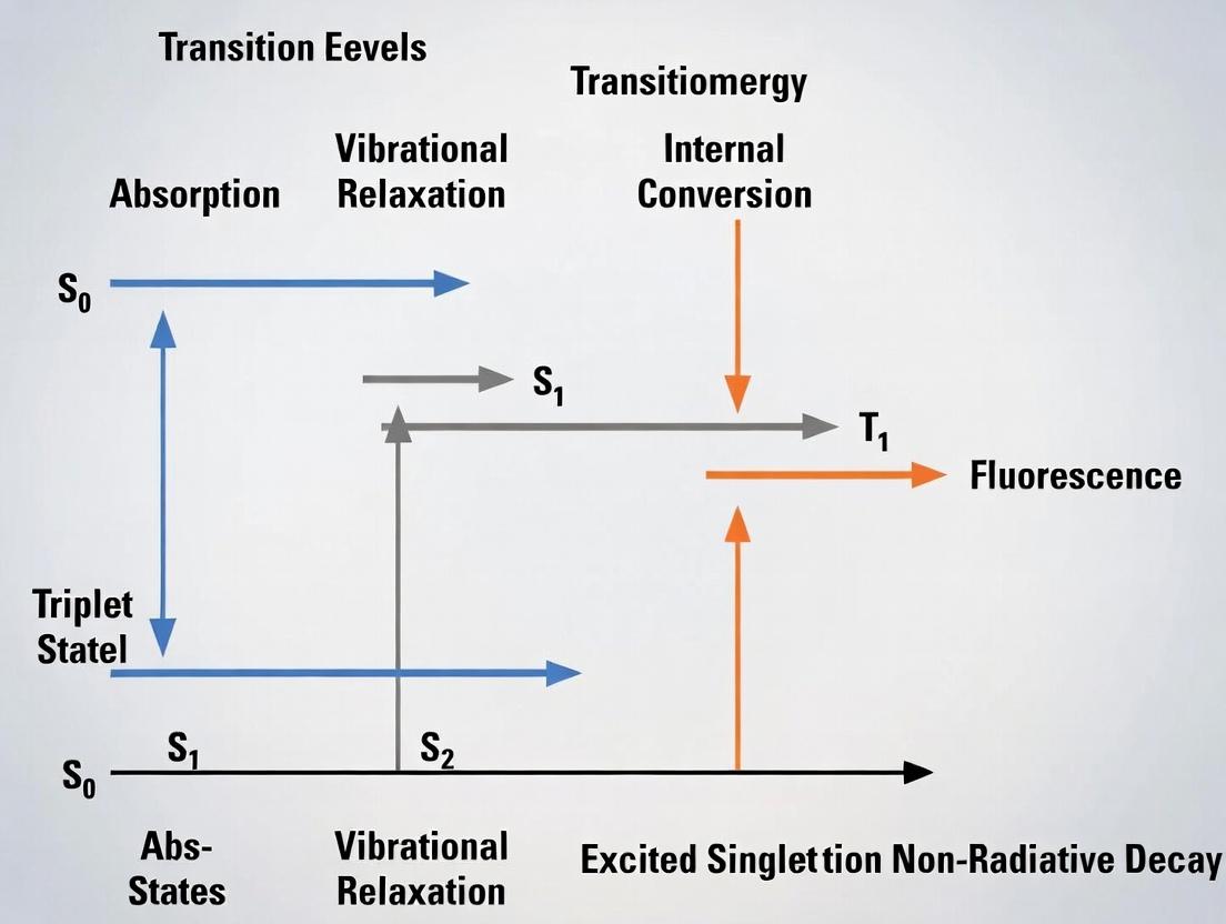
Within the canonical Jablonski diagram explanation of molecular photophysics, fluorescence lifetime (τ) is a fundamental parameter defined as the average time a molecule spends in the excited electronic state (typically S₁) before returning to the ground state (S₀) via the emission of a photon. It represents the natural decay time constant of the excited-state population in the absence of non-radiative processes. Formally, for a population of identical fluorophores excited instantaneously, the fluorescence intensity decay I(t) is described by I(t) = I₀ * exp(-t/τ), where τ is the fluorescence lifetime. This parameter is intrinsic to the fluorophore but is modulated by its immediate molecular environment, making it a powerful tool in biophysical research and drug development for probing molecular interactions, conformational changes, and local physicochemical properties.

Recent research highlights key fluorescence lifetime ranges for common fluorophores and biological phenomena.

Table 1: Fluorescence Lifetimes of Common Biological Fluorophores and Labels

Fluorophore	Typical Lifetime Range (ns)	Primary Application	Key Environmental Sensitivity
NAD(P)H (free)	0.3 - 0.5	Cellular metabolism	Protein binding
NAD(P)H (bound)	1.0 - 3.5	Cellular metabolism	Binding conformation
FAD (Flavin)	2.0 - 4.0	Cellular metabolism	Redox state, quenching
GFP (e.g., EGFP)	2.4 - 2.7	Protein tagging & localization	pH, Cl⁻ concentration
Tryptophan (protein)	1.0 - 6.0	Protein structure	Solvent exposure, quenching
Cyanine dyes (e.g., Cy3)	0.3 - 0.5	Nucleic acid/protein labeling	Local rigidity, FRET
Ruthenium complexes	200 - 1000	Oxygen sensing	O₂ quenching
Lanthanides (e.g., Eu³⁺)	10⁵ - 10⁶ (µs-ms)	TR-FRET assays	Protected from aqueous quenching

Table 2: Impact of Common Environmental Factors on Fluorescence Lifetime

Environmental Factor	Typical Direction of τ Change	Typical Magnitude of Change	Primary Mechanism
Increased Temperature	Decrease	~1-5% per 10°C	Enhanced non-radiative decay
Quencher (e.g., O₂, I⁻)	Decrease	Up to 100% (to zero)	Dynamic (collisional) quenching
Viscosity Increase	Increase	Up to 200%+	Restriction of non-radiative motions
FRET Occurrence	Decrease	Up to 100% (to zero)	Energy transfer to acceptor
Polarity Change	Variable (Increase/Decrease)	10-50%	Solvent relaxation, ICT states

Key Experimental Methodologies

Time-Correlated Single Photon Counting (TCSPC)

TCSPC is the gold-standard method for precise lifetime determination.

Protocol:

• Excitation: A pulsed laser source (e.g., Ti:Sapphire, diode laser) with a repetition rate (1-80 MHz) and pulse width much shorter (<100 ps) than the expected lifetime excites the sample.
• Detection: A single-photon-sensitive detector (e.g., Microchannel Plate Photomultiplier Tube - MCP-PMT, or Single-Photon Avalanche Diode - SPAD) detects emitted photons.
• Timing: For each detected photon, the time difference between the laser pulse (start signal) and photon arrival (stop signal) is measured by a high-precision timing discriminator and time-to-digital converter (TDC).
• Histogramming: These time differences are accumulated over millions of pulses to build a histogram representing the fluorescence decay curve I(t).
• Analysis: The histogram is fitted, typically using iterative reconvolution with the instrument response function (IRF) and a decay model (e.g., multi-exponential, stretched exponential), to extract lifetime components (τᵢ) and their amplitudes (αᵢ).

Frequency-Domain Fluorescence Lifetime Imaging Microscopy (FD-FLIM)

FD-FLIM is widely used for rapid lifetime imaging in live cells.

Protocol:

• Excitation: The sample is excited with intensity-modulated light (sinusoidally, at radio frequencies, e.g., 10-200 MHz), typically from a modulated diode laser or a CW laser whose beam is passed through an electro-optic modulator (EOM).
• Detection: The emitted fluorescence, which is also modulated but phase-shifted (Δφ) and demodulated (demodulation factor, m), is detected.
• Measurement: A gain-modulated image intensifier in front of a CCD or sCMOS camera is used as a detector. The intensifier's gain is modulated at the same frequency as the excitation, with a variable phase offset.
• Data Acquisition: Images are captured at multiple (typically 4-12) phase offsets between the excitation and detector modulation. Alternatively, the phase and modulation can be measured directly with homodyne or heterodyne detection schemes.
• Analysis: For each pixel, the phase shift (Δφ) and demodulation (m) relative to the excitation are calculated. The lifetime is computed from these values: τφ = (1/ω)tan(Δφ) and τm = (1/ω)√(1/m² - 1), where ω is the angular modulation frequency. These are equal for single-exponential decays.

Time-Gated FLIM (TG-FLIM)

A simpler, robust method suitable for longer-lived fluorophores.

Protocol:

• Excitation & Detection: The sample is excited with a pulsed laser. A gated optical intensifier (GOI) or a gated camera acts as a fast shutter in front of the detector.
• Gating: Multiple images are captured, each within a specific short time window (gate) delayed after the excitation pulse. Typically, at least two gates are used (e.g., one early, one late).
• Calculation: For a two-gate system with intensities I₁ and I₂ in gates centered at times t₁ and t₂ after the pulse, the lifetime can be approximated as τ = (t₂ - t₁) / ln(I₁/I₂), assuming a single-exponential decay.
• Analysis: More sophisticated multi-gate fitting improves accuracy and allows for multi-exponential analysis.

Visualization of Core Concepts

Title: Jablonski Diagram with Lifetime Timescales

Title: TCSPC Instrumentation Workflow

Title: Environmental Factors Affecting Lifetime

The Scientist's Toolkit: Key Research Reagent Solutions

Table 3: Essential Materials for Fluorescence Lifetime Experiments

Item	Function/Brief Explanation	Example Product/Note
Fluorescent Labels/Dyes	Site-specific tagging of biomolecules for lifetime measurement.	HaloTag ligands with Janelia Fluor dyes (long τ, bright), Cy dyes, ATTO dyes. Choose based on lifetime range and environmental sensitivity.
FRET Pairs	For measuring molecular proximity via donor lifetime reduction.	e.g., GFP (Donor) / mCherry (Acceptor) for proteins; Cy3 (Donor) / Cy5 (Acceptor) for nucleic acids.
Lifetime Reference Standard	To measure and correct for the instrument response function (IRF).	A fluorophore with a known, single-exponential, short lifetime (e.g., Fluorescein in pH 11 buffer, τ ~4.0 ns; Rose Bengal, τ ~0.1 ns).
Quenching Agents	To validate dynamic quenching effects on lifetime.	Potassium Iodide (KI) for collisional quenching of tryptophan; Sodium dithionite for reducing flavins.
Oxygen Scavenging System	To remove O₂ (a potent quencher) for longer, more stable measurements.	Glucose Oxidase/Catalase with glucose; Protocatechuate Dioxygenase (PCD)/Protocatechuic Acid (PCA) for single-molecule studies.
Mounting Media for FLIM	To preserve sample state and minimize environmental artifacts during imaging.	ProLong Glass/Live Antifade reagents; Glycerol-based media with anti-bleaching agents; Phenol-red free live-cell imaging medium.
FLIM-Compatible Cell Culture Substrates	Provide low background autofluorescence and high optical clarity.	Glass-bottom dishes (e.g., #1.5 coverslip thickness) with poly-D-lysine or collagen coating; Quartz substrates for UV FLIM.
Metal-Enhanced Fluorescence (MEF) Substrates	To study plasmonic effects on lifetime (dramatic reduction).	Gold or silver nanoparticle films or patterned nanostructures.
Lanthanide Chelates & Cryptates	For time-resolved FRET (TR-FRET) assays, leveraging their very long (µs-ms) lifetimes.	Eu³⁺/Tb³⁺ cryptates from Cisbio or PerkinElmer; LanthaScreen tags from Thermo Fisher.

This whitepaper, framed within the broader thesis of Jablonski diagram-driven fluorescence lifetime research, details the fundamental equations that connect the experimentally measurable fluorescence lifetime (τ) to the intrinsic molecular rate constants for radiative (kᵣ) and non-radiative (k_nr) decay. This relationship is central to quantitative spectroscopy and its applications in drug development, where it serves as a sensitive probe for molecular environment, conformation, and binding events.

Core Theoretical Framework

The photophysical pathways of a fluorophore, as depicted in the Jablonski diagram, are governed by first-order kinetics. Upon excitation to a higher electronic singlet state (S₁, S₂), a molecule rapidly relaxes to the lowest vibrational level of S₁. From there, it returns to the ground state (S₀) via several competing pathways, primarily:

• Radiative decay: Emission of a photon (fluorescence).
• Non-radiative decay: Internal conversion, releasing energy as heat.

The fluorescence lifetime (τ) is defined as the average time a molecule spends in the excited state before returning to the ground state. It is the inverse of the total decay rate from the excited state.

The Fundamental Equation

The fluorescence lifetime (τ) is inversely proportional to the sum of all rate constants depleting the excited state:

τ = 1 / (kᵣ + k_nr)

Where:

• τ = Observed fluorescence lifetime (seconds, typically ns).
• kᵣ = Radiative rate constant (s⁻¹).
• k_nr = Non-radiative rate constant (s⁻¹).

Derived Relationships: Quantum Yield and Intensity

The fluorescence quantum yield (Φ), defined as the fraction of excited molecules that decay via photon emission, is given by:

Φ = kᵣ / (kᵣ + k_nr)

Combining the equations for τ and Φ yields two critical relationships:

Φ = kᵣ · τ kᵣ = Φ / τ k_nr = (1/τ) - kᵣ = (1 - Φ) / τ

These equations allow researchers to deconvolve the individual rate constants from experimental measurements of lifetime and quantum yield, providing direct insight into molecular efficiency and competing decay processes.

Table 1: Summary of Key Equations and Parameters

Parameter	Symbol	Defining Equation	Relationship to Lifetime (τ)
Fluorescence Lifetime	τ	τ = 1 / (kᵣ + k_nr)	Measured directly (e.g., via TCSPC).
Quantum Yield	Φ	Φ = kᵣ / (kᵣ + k_nr)	Φ = kᵣ · τ
Radiative Rate Constant	kᵣ	kᵣ = Φ / τ	Derived from Φ and τ.
Non-Radiative Rate Constant	k_nr	k_nr = (1 - Φ) / τ	Derived from Φ and τ.

Experimental Protocols for Determining τ, Φ, kᵣ, and k_nr

Time-Correlated Single Photon Counting (TCSPC) for Lifetime (τ)

Principle: The most precise method for measuring fluorescence lifetime. It builds a histogram of delays between an excitation laser pulse and the detection of the first emitted photon.

Detailed Protocol:

• Sample Preparation: Dilute fluorophore in desired solvent/buffer to an optical density < 0.1 at excitation wavelength to avoid inner filter effects and aggregation.
• Instrument Setup:
  • Excitation Source: Use a pulsed diode laser or Ti:Sapphire laser with pulse width << τ.
  • Detector: Employ a fast microchannel plate photomultiplier tube (MCP-PMT) or single-photon avalanche diode (SPAD).
  • Electronics: Connect to a constant fraction discriminator (CFD) and time-to-amplitude converter (TAC).
• Data Acquisition: Collect photons until the histogram peak reaches ~10⁴ counts. Maintain a low count rate (<1% of laser repetition rate) to avoid pulse pile-up.
• Data Analysis: Fit the decay histogram I(t) to a multi-exponential model: I(t) = Σ αᵢ exp(-t/τᵢ), where αᵢ are amplitudes and τᵢ are lifetimes. Use iterative reconvolution with the instrument response function (IRF) for accuracy.

Integrating Sphere Method for Absolute Quantum Yield (Φ)

Principle: Measures the total number of photons emitted versus the total number of photons absorbed by the sample.

Detailed Protocol:

• Setup: Place the sample (in a quartz cuvette) at the center of a calibrated integrating sphere coated with Spectralon.
• Excitation: Use a monochromated CW light source (e.g., xenon lamp) or a known wavelength laser.
• Measurement Sequence: a. Record emission spectrum with sample in place and excitation beam hitting the sample directly. b. Record emission spectrum with an empty cuvette or a non-absorbing scatterer (e.g., Ludox) in place, with the beam hitting the same spot. This measures the incident excitation profile.
• Calculation: Φ = (Es - E0) / (L0 - Ls), where Es and E0 are integrated emissions from the sample and blank, respectively, and L0 and Ls are integrated excitation profiles measured for the blank and sample, respectively.

Table 2: Experimental Data for a Model Fluorophore (Rhodamine 6G in Ethanol)

Parameter	Measured Value	Method/Instrument	Calculated Rate Constants
Lifetime (τ)	3.9 ns	TCSPC (405 nm laser, SPAD)	--
Quantum Yield (Φ)	0.94	Integrating Sphere + Fluorometer	--
Radiative kᵣ	2.41 x 10⁸ s⁻¹	kᵣ = Φ / τ	(0.94 / 3.9e-9 s)
Non-Radiative k_nr	1.54 x 10⁷ s⁻¹	k_nr = (1 - Φ) / τ	(0.06 / 3.9e-9 s)

Visualization of Kinetics and Pathways

Diagram 1: Jablonski Kinetics & Rate Constants

Diagram 2: Workflow to Extract kᵣ and k_nr

The Scientist's Toolkit: Essential Research Reagents & Materials

Table 3: Key Research Reagent Solutions for Fluorescence Lifetime Studies

Item	Function & Explanation
Reference Fluorophores	Compounds with well-characterized, stable lifetimes (e.g., Coumarin 6, Rhodamine 6G, Fluorescein). Used for instrument calibration and validation.
Degassed Solvents	Solvents (e.g., ethanol, cyclohexane) purged of oxygen via freeze-pump-thaw cycles. Oxygen is a potent quencher that reduces τ; its removal allows measurement of intrinsic kᵣ and k_nr.
Buffer Systems	Phosphate (PBS), Tris, or HEPES buffers for biologically relevant measurements. Ionic strength and pH must be controlled as they can affect fluorophore τ and Φ.
Quenchers	Compounds like potassium iodide (KI) or acrylamide. Selectively increase k_nr via collisional quenching. Used in Stern-Volmer experiments to probe fluorophore accessibility.
Oxygen Scavenging Systems	Enzymatic (e.g., glucose oxidase/catalase) or chemical (e.g., Trolox) systems to remove dissolved oxygen in live-cell or prolonged measurements, preventing photobleaching and quenching.
Viscogens	Reagents like glycerol or sucrose used to vary solvent viscosity. Affects rotational diffusion and can modulate k_nr for some quenching mechanisms.
Cuvettes	High-quality, fluorescence-grade quartz cuvettes with all four optical faces polished. Essential for minimizing scatter and background in lifetime and quantum yield measurements.

Within the framework of Jablonski diagram-based fluorescence lifetime research, the measured lifetime of a fluorophore is not an immutable property. The intrinsic lifetime (τ₀) is the natural radiative lifetime in the absence of non-radiative decay pathways. In contrast, the apparent lifetime (τ) is the experimentally measured value, heavily modulated by the probe's local microenvironment. This whitepaper elucidates the physical principles governing this distinction, details experimental methodologies for its investigation, and discusses its critical implications for biomedical research and drug development.

Fundamental Principles: A Jablonski Diagram Perspective

The Jablonski diagram provides the foundational model for understanding fluorescence phenomena. The intrinsic lifetime is derived from the rate of radiative decay ((kr)) from the first excited singlet state (S₁) to the ground state (S₀): τ₀ = 1 / (kr). However, in real systems, competing non-radiative processes ((k{nr}))—such as internal conversion, vibrational relaxation, and dynamic quenching—deplete the excited state population. The apparent lifetime is thus given by τ = 1 / ((kr + k_{nr})).

The microenvironment influences (k_{nr}) through multiple mechanisms:

• Collisional Quenching: Dynamic interactions with solutes like oxygen, halides, or heavy metals.
• Solvent Effects: Polarity, viscosity, and refractive index alter the fluorophore's energy states and rotational freedom.
• Förster Resonance Energy Transfer (FRET): Non-radiative energy transfer to an acceptor molecule, drastically shortening the donor's apparent lifetime.
• Binding Interactions: Changes in local dielectric constant or restriction of motion upon binding to a target.

The relationship between intrinsic and apparent lifetime, and quantum yield (Φ), is: Φ = (kr) / ((kr + k_{nr})) = τ / τ₀.

Quantitative Comparison of Influencing Factors

The following table summarizes key microenvironmental factors and their typical quantitative impact on apparent fluorescence lifetime.

Table 1: Microenvironmental Factors Modulating Apparent Fluorescence Lifetime

Factor	Mechanism	Typical Impact on τ	Example System/Probe
Oxygen Concentration	Collisional quenching (Triplet state interaction)	Decrease: ~20-50% from anoxic to air-saturated	Ruthenium complexes, Pyrene
Halide Ion (Cl⁻, I⁻)	Collisional quenching (Heavy atom effect)	Decrease: Can reduce τ by >90% at high [quencher]	Quinine sulfate, Certain GFP mutants
Solvent Polarity	Stabilization/destabilization of excited state	Increase or Decrease: Varies by probe; can shift by nanoseconds	Prodan, LAURDAN
Solvent Viscosity	Restriction of intramolecular rotation (RICT)	Increase: Often 2-5 fold increase from water to glycerol	Molecular rotors (e.g., CCVJ)
FRET Efficiency (E)	Non-radiative energy transfer	Decrease: τDonor(app) = τDonor * (1 - E)	GFP-RFP FRET pairs (e.g., CFP-YFP)
pH	Protonation/deprotonation of fluorophore	Biphasic change: Specific to probe pKa	Fluorescein, SNARF
Temperature	Increased vibrational quenching	Decrease: ~1-3% per °C (varies widely)	Most organic dyes

Experimental Protocols for Decoupling Intrinsic and Apparent Lifetime

Protocol 3.1: Time-Correlated Single Photon Counting (TCSPC) for Lifetime Measurement

Objective: To measure the apparent fluorescence lifetime (τ) of a sample with high precision.

• Sample Preparation: Prepare the fluorophore in the microenvironment of interest (e.g., buffer, cells, tissue). Include a reference dye with known lifetime (e.g., Rhodamine B in water, τ ≈ 1.68 ns) for instrument response function (IRF) validation.
• Instrument Setup: Use a TCSPC system with pulsed laser excitation (e.g., 405 nm, 80 MHz repetition rate), a fast photomultiplier tube (PMT) or microchannel plate (MCP) detector, and TCSPC electronics.
• Data Acquisition: Collect photons until a peak count of 10,000-20,000 is achieved in the decay profile maximum to ensure good signal-to-noise ratio.
• Data Analysis: Fit the decay curve (I(t)) to a multi-exponential model: (I(t) = \sumi αi \exp(-t/τi)), where (αi) are amplitudes and (τ_i) are lifetime components. Use iterative reconvolution with the IRF for accurate fitting.

Protocol 3.2: Determining Intrinsic Lifetime (τ₀)

Objective: To estimate the intrinsic radiative lifetime, which is often not directly measurable.

• Method 1: Using Quantum Yield and Apparent Lifetime: Measure the absolute fluorescence quantum yield (Φ) of the fluorophore in a non-quenching, rigid environment (e.g., low temperature, rigid matrix). Measure its apparent lifetime (τ) in the same condition. Calculate τ₀ = τ / Φ.
• Method 2: Strickler-Berg Analysis: Record the absorption and fluorescence emission spectra of the fluorophore in a dilute solution. Apply the Strickler-Berg equation, which relates the integrated absorption coefficient to the radiative rate constant (kr), to calculate τ₀ = 1/(kr).

Protocol 3.3: Mapping Microenvironment Viscosity via FLIM

Objective: To use apparent lifetime as a quantitative readout of local viscosity using a molecular rotor.

• Probe Selection: Use a viscosity-sensitive fluorophore (e.g., BODIPY-based molecular rotor).
• Calibration: Prepare a series of glycerol-water mixtures (0-99% w/w) of known viscosity. Acquire fluorescence lifetime images (FLIM) of the rotor in each mixture using a multiphoton or confocal FLIM microscope. Plot τ vs. viscosity to create a calibration curve.
• Biological Application: Incubate live cells with the cell-permeable rotor. Acquire FLIM data under identical instrument settings.
• Analysis: Convert the measured apparent lifetime at each pixel to a viscosity map using the calibration curve.

Visualizing Key Concepts and Pathways

Title: Jablonski Diagram Showing Decay Pathways

Title: Relationship Between τ₀, τ, and the Microenvironment

The Scientist's Toolkit: Key Reagent Solutions

Table 2: Essential Research Reagents for Fluorescence Lifetime Studies

Reagent / Material	Function & Rationale
Lifetime Reference Dyes (e.g., Fluorescein in 0.1M NaOH, τ ~4.0 ns; Rhodamine 6G in water)	Used to measure the Instrument Response Function (IRF) and validate TCSPC/FLIM system performance. Provides a known lifetime standard.
Quenching Agents (Potassium Iodide, Acrylamide, Sodium Sulfide)	To selectively and dynamically quench fluorescence, allowing study of solvent accessibility and calculation of Stern-Volmer constants.
Molecular Rotor Probes (e.g., CCVJ, DCVJ, BODIPY-FL-C₁₂)	Viscosity-sensitive fluorophores whose non-radiative decay rate depends on intramolecular rotation, making apparent lifetime a direct measure of local microviscosity.
Environment-Sensitive Probes (Prodan, LAURDAN, ANS)	Fluorophores whose emission spectrum and lifetime shift dramatically with solvent polarity/packaging, useful for membrane and protein folding studies.
FRET Pair Standards (e.g., CFP-YFP linked constructs with known spacers)	Validated donor-acceptor pairs with characterized Förster distance (R₀) to calibrate FLIM-FRET measurements and quantify molecular interactions.
Deoxygenation Kits (Glucose Oxidase/Catalase, Nitrogen/Argon Sparging Systems)	To remove molecular oxygen (a potent triplet state quencher) from solutions, allowing measurement of unquenched lifetimes and studying oxygen-sensitive probes.
Viscosity Calibration Kits (Glycerol/Water, Sucrose/Water mixtures)	Pre-measured mixtures of known viscosity for calibrating the response of molecular rotors or other viscosity-sensitive probes.
Phase Transition Lipids (DMPC, DPPC, Cholesterol)	For constructing model membranes (vesicles, SLBs) of defined composition and phase (gel/fluid) to study lipid order and protein-lipid interactions via lifetime changes.

Within the framework of fluorescence research grounded in the Jablonski diagram, the fluorescence lifetime (τ) emerges as a fundamentally more robust parameter than fluorescence intensity. The Jablonski diagram illustrates the electronic state transitions: absorption (excitation), vibrational relaxation, and emission, including non-radiative decay pathways. While intensity is the observable output, it is the lifetime—the average time a molecule spends in the excited state before returning to the ground state—that provides intrinsic, quantitative insights into the molecular microenvironment, independent of many confounding variables that plague intensity-based measurements.

Core Advantages of Lifetime over Intensity Measurements

Fluorescence intensity is a population-based measurement, dependent on the number of emitting fluorophores and the efficiency of photon collection. It is susceptible to numerous artifacts: variations in excitation light source power, fluorophore concentration, optical path length, sample turbidity, photobleaching, and detector sensitivity. These factors make quantitative, comparative intensity measurements challenging.

In contrast, fluorescence lifetime is an intrinsic molecular property of the fluorophore in its specific environment. It is defined as the inverse of the sum of the radiative ((kr)) and non-radiative ((k{nr})) decay rates from the excited state: τ = 1 / (kr + k{nr}). This lifetime is sensitive to molecular interactions, such as Förster Resonance Energy Transfer (FRET), quenching, changes in local pH, viscosity, temperature, and ion concentration, but is inherently independent of fluorophore concentration and excitation intensity. This makes Fluorescence Lifetime Imaging Microscopy (FLIM) a powerful quantitative tool.

Quantitative Comparison of Key Parameters

The following table summarizes the fundamental differences between intensity-based and lifetime-based measurements.

Table 1: Key Characteristics of Fluorescence Intensity vs. Lifetime Measurements

Parameter	Fluorescence Intensity	Fluorescence Lifetime (τ)
Dependence on Fluorophore Concentration	Linear (Direct)	None
Dependence on Excitation Intensity	Linear (Direct)	None
Quantitative Robustness	Low - Highly variable due to instrumental and sample factors	High - Intrinsic property of the fluorophore's environment
Primary Environmental Sensitivities	Indirect via concentration changes	Direct via changes in (k_{nr}) (quenching, FRET, viscosity, pH)
Susceptibility to Photobleaching	High (Signal loss)	Low (Can measure population heterogeneity)
Key Measurement Modality	Steady-state	Time-domain (pulse excitation) or Frequency-domain (modulated excitation)

Table 2: Common FLIM Applications and Their Lifetime Ranges

Application / Phenomenon	Typical Lifetime Change	Molecular Information Probed
FRET (Donor)	Decrease (e.g., 2.8 ns → 1.2 ns)	Protein-protein interactions, conformational changes (<10 nm)
Collisional Quenching	Decrease (Stern-Volmer kinetics)	Molecular accessibility, dynamic quenching events
Ion Concentration (e.g., Ca²⁺ with dyes)	Increase or Decrease (specific to dye)	Ion binding and cellular signaling
Microviscosity (e.g., with molecular rotors)	Increase with viscosity	Local membrane order, cytoplasmic crowding
pH Sensing (with rationetric dyes)	Change with protonation	Local pH, organelle acidity

Detailed Experimental Protocols

Protocol 1: Time-Correlated Single Photon Counting (TCSPC) for FLIM

Objective: To measure the fluorescence lifetime decay curve at each pixel of an image.

• Sample Preparation: Label cells or tissue with a suitable fluorophore (e.g., GFP fusion protein, synthetic dye). Mount on microscope stage.
• Instrument Setup: Use a confocal or multiphoton microscope equipped with a pulsed laser (e.g., Ti:Sapphire, ~80 MHz repetition rate, pulse width <100 fs), high-sensitivity detectors (e.g., hybrid PMT, SPAD), and TCSPC electronics.
• Data Acquisition:
  • The pulsed laser excites the sample. Each detected photon is timestamped relative to the laser pulse.
  • Photons are accumulated over millions of laser pulses to build a histogram of photon arrival times at each pixel, which represents the fluorescence decay curve (I(t)).
• Data Analysis: Fit the decay curve (I(t)) at each pixel to a multi-exponential model: (I(t) = \sumi αi exp(-t/τi)), where (αi) is the amplitude and (τ_i) is the lifetime of component i. Generate a lifetime map (FLIM image).

Protocol 2: FLIM-FRET Assay for Protein-Protein Interaction

Objective: To quantify protein-protein interaction in live cells via donor fluorescence lifetime change.

• Construct Design: Create fusion proteins: Protein A tagged with a donor fluorophore (e.g., mCerulean, lifetime ~3.8 ns) and Protein B tagged with an acceptor fluorophore (e.g., mVenus).
• Sample Preparation: Co-transfect cells with donor-only and donor+acceptor constructs. Include a donor-only control.
• FLIM Acquisition: Perform TCSPC-FLIM on the donor channel (excite donor, collect donor emission). Acquire images of donor-only and donor+acceptor cells.
• Analysis & Quantification:
  • Fit donor lifetimes in control cells to obtain the unquenched donor lifetime (τD).
  • Fit donor lifetimes in cells expressing both donor and acceptor. A decrease in τ indicates FRET.
  • Calculate the FRET efficiency: (E = 1 - (τ{DA} / τD)), where (τ{DA}) is the donor lifetime in the presence of acceptor.
  • Generate an Efficiency map to visualize spatial interaction heterogeneity.

Essential Visualization of Concepts and Workflows

Title: Jablonski Diagram with Lifetimes

Title: Factors Affecting Intensity vs Lifetime

Title: FLIM-FRET Experimental Workflow

The Scientist's Toolkit: Key Reagent Solutions for FLIM Research

Table 3: Essential Research Reagents and Materials for FLIM

Item / Reagent	Function / Role in FLIM Experiments
Genetically Encoded Biosensors (e.g., mCerulean3, mClover3)	Donor/Acceptor pairs with long, mono-exponential lifetimes, ideal for reliable FLIM-FRET in live cells.
Environment-Sensing Dyes (e.g., FLIM pH probes, Molecular Rotors)	Probes whose lifetime changes in response to specific microenvironmental parameters (pH, viscosity, ions).
TCSPC-Compatible Pulsed Laser	Provides the precise, high-repetition-rate excitation pulses required for time-domain lifetime measurement.
High Quantum Efficiency Detector (Hybrid PMT, SPAD array)	Maximizes photon detection efficiency for faster acquisition and better signal-to-noise in lifetime decays.
FLIM Analysis Software (e.g., SPCImage, TRI2, FLIMfit)	Enables fitting of complex decay models, phasor analysis, and generation of lifetime parameter maps.
Reference Fluorophore (e.g., Fluorescein, Coumarin 6)	Standards with well-characterized lifetimes for instrument calibration and validation.
Mounting Media with Anti-fading Agents	Preserves fluorescence signal and minimizes photobleaching during prolonged imaging sessions.

From Theory to Bench: FLIM, FRET, and Quantitative Applications in Biomedical Research

The Jablonski Diagram and Fluorescence Lifetime Foundation

Fluorescence Lifetime Imaging Microscopy (FLIM) is a powerful quantitative imaging technique that maps the spatial distribution of fluorescent species based on their excited-state decay rates, or lifetimes (τ). This lifetime is an intrinsic molecular property, largely independent of fluorophore concentration, excitation intensity, and light scattering, making it a robust reporter of the local biochemical microenvironment. Its fundamental principles are rooted in the Jablonski diagram, which describes the electronic state transitions of a fluorophore. Within this diagram, fluorescence lifetime is defined as the average time a molecule spends in the excited singlet state (S1) before returning to the ground state (S0) via photon emission. The lifetime is typically on the order of picoseconds to nanoseconds.

Crucially, the fluorescence lifetime is highly sensitive to factors that affect the fluorophore's electronic structure, including:

• Förster Resonance Energy Transfer (FRET): A non-radiative energy transfer to an acceptor molecule, which shortens the donor's lifetime, enabling the study of molecular interactions.
• Local Environment: Parameters such as pH, ion concentration (e.g., Ca²⁺, Cl⁻), viscosity, temperature, and oxygen saturation (quenching) can alter decay kinetics.
• Molecular Conformation/Binding: Changes in the fluorophore's immediate chemical environment upon binding or conformational change can affect τ.

Thus, FLIM transcends mere localization, providing functional insight into molecular interactions, conformation, and the cellular microenvironment, forming a critical pillar of modern fluorescence research.

Core FLIM Modalities

The two primary techniques for measuring fluorescence lifetime are Time-Correlated Single Photon Counting (TCSPC) and Frequency-Domain FLIM (FD-FLIM). They offer complementary approaches to sampling the fluorescence decay curve.

Time-Correlated Single Photon Counting (TCSPC)

TCSPC is a time-domain method considered the gold standard for its high accuracy and precision. It operates on the principle of recording the arrival time of individual photons relative to a pulsed excitation laser.

Experimental Protocol:

• Excitation: A high-repetition-rate pulsed laser (e.g., picosecond diode laser, Ti:Sapphire) illuminates the sample.
• Detection: A single-photon-sensitive detector, such as a photomultiplier tube (PMT) or hybrid detector, detects emitted photons.
• Timing: For each detected photon, a time-to-amplitude converter (TAC) or a time-to-digital converter (TDC) measures the delay between the laser pulse (start signal) and the photon arrival (stop signal).
• Histogramming: This delay time is recorded, and over millions of pulses, a histogram of photon counts versus arrival time is built, which directly represents the fluorescence decay curve.
• Analysis: The decay curve is fitted to an exponential model (e.g., ( I(t) = \sumi αi \exp(-t/τ_i) )) to extract lifetime components (τi) and their amplitudes (αi).

Key Characteristics:

• Sequential Acquisition: Builds the decay curve photon-by-photon; best suited for static or slow dynamic processes.
• High Temporal Resolution: Can resolve multi-exponential decays with high precision.
• Slow Imaging: Acquisition speed is limited by the count rate (typically 1-10% of laser pulse rate to avoid pile-up distortion).

Table 1: Key TCSPC System Parameters and Typical Values

Parameter	Typical Specification	Function/Role
Pulsed Laser	1-100 MHz rep rate, <100 ps pulse width	Provides the "start" timing reference
Detector	PMT, Hybrid PMT, SPAD	Provides the "stop" signal for single photons
TCSPC Module	TAC/TDC, Router (for multi-channel)	Measures time delay between start and stop
Count Rate	1-10% of laser repetition rate	Prevents "pile-up" distortion of decay curve
Temporal Resolution	< 10 ps (system dependent)	Ability to distinguish fast lifetime components

Diagram: TCSPC Timing and Data Acquisition Workflow

Frequency-Domain FLIM (FD-FLIM)

FD-FLIM operates in the frequency domain. The sample is excited with intensity-modulated light (typically a sinusoidally modulated continuous-wave laser or a pulsed laser with modulated gain). The emitted fluorescence is also modulated at the same frequency but is phase-shifted (Δφ) and demodulated (modulation depth, M) relative to the excitation.

Experimental Protocol:

• Modulated Excitation: The intensity of the excitation light is sinusoidally modulated at a radio frequency (ω, typically 10-300 MHz).
• Detection & Analysis: The emitted fluorescence signal, captured by a detector (often a gain-modulated image intensifier coupled to a CCD/CMOS camera), is analyzed to determine:
  • Phase Shift (Δφ): The time delay between excitation and emission waveforms.
  • Modulation (M): The ratio of the AC amplitude to the DC offset of the emission relative to that of the excitation.
• Lifetime Calculation: The lifetime can be calculated from these two independent measurements at each pixel:
  • Phase Lifetime: τφ = (1/ω) * tan(Δφ)
  • Modulation Lifetime: τM = (1/ω) * √((1/M²) - 1) For a single exponential decay, τφ = τM.

Key Characteristics:

• Parallel Acquisition: Can capture lifetime information from all pixels in an image simultaneously using a camera.
• High Speed: Well-suited for live-cell imaging and dynamic processes.
• Lifetime Precision: Generally lower than TCSPC for the same acquisition time, especially for complex decays.

Table 2: Comparison of TCSPC and FD-FLIM Modalities

Feature	TCSPC-FLIM	FD-FLIM
Acquisition Domain	Time Domain	Frequency Domain
Speed	Slower (photon-limited)	Faster (camera-based)
Temporal Precision	Very High	Moderate to High
Ideal For	High-precision kinetics,multi-exponential analysis	Fast dynamic processes,high-throughput screening
Excitation Source	Pulsed Laser	Intensity-Modulated Light
Primary Detector	Point Detectors (PMT)	Modulated Image Intensifier + Camera
Data Output	Photon Arrival Time Histogram	Phase Shift (Δφ) & Modulation (M) Images

Diagram: FD-FLIM Signal Modulation and Detection Workflow

The Scientist's Toolkit: Key Research Reagent Solutions

Table 3: Essential Materials for FLIM Experiments

Item	Function & Role in FLIM
Fluorescent Probes with Environment-Sensitive Lifetimes	e.g., NAD(P)H, FAD (autofluorescence, metabolic sensing); Ruthenium complexes (oxygen sensing); pHluorins (pH sensing). Lifetime reports on specific biochemical parameters.
FRET Pairs (Donor & Acceptor)	e.g., CFP/YFP, GFP/mCherry, organic dye pairs (ATTO dyes, Cy dyes). Donor lifetime shortening is a direct, quantitative measure of FRET efficiency and molecular proximity (<10 nm).
FLIM-Compatible Fixation & Mounting Media	Media that do not autofluoresce or quench fluorescence in the relevant lifetime range (e.g., ProLong Diamond, specific glycerol-based media). Critical for preserving lifetime signatures.
Lifetime Reference Standards	Dyes or materials with known, stable single-exponential lifetimes (e.g., Fluorescein in pH 9 buffer, Rose Bengal, quantum dot samples). Essential for system calibration and validation.
Specialized Cell Culture Substrates	Glass-bottom dishes or #1.5 coverslips with high UV/visible transmission and minimal autofluorescence. Thickness is critical for objective correction.
Time-Resolved Analysis Software	Software for decay curve fitting (e.g., SPCImage, TRI2, FLIMfit), phasor analysis, and lifetime component separation. Enables quantitative interpretation of FLIM data.

Fluorescence Lifetime (FLT) imaging microscopy (FLIM) provides a robust, quantitative method for probing the local biochemical microenvironment of fluorophores. Unlike intensity-based measurements, FLT is an intrinsic property of a fluorophore that is independent of concentration, photobleaching within limits, and excitation light intensity, but exquisitely sensitive to its immediate surroundings. This technical guide details the application of FLT as a sensor for key physiological parameters—pH, ion concentration, oxygenation, and molecular crowding—framed within the foundational context of the Jablonski diagram and photophysical principles.

Photophysical Foundation: The Jablonski Diagram and Fluorescence Lifetime

Fluorescence originates from the radiative relaxation of an excited singlet state (S1) to the ground state (S0). The Jablonski diagram illustrates competing pathways for depopulation of S1: radiative fluorescence and non-radiative processes (e.g., internal conversion, quenching). The average time a fluorophore spends in the excited state is its fluorescence lifetime (τ).

[ \tau = \frac{1}{kr + k{nr}} ]

where ( kr ) is the radiative decay rate and ( k{nr} ) is the sum of all non-radiative decay rates. Any environmental factor that modulates ( k_{nr} ) (e.g., via collisional quenching, energy transfer, or changes in the fluorophore's electronic structure) will alter τ. This principle forms the basis for FLT-based sensing.

Diagram 1: Jablonski diagram with environmental quenching.

FLT Sensing Mechanisms and Quantitative Probes

Table 1: FLT Sensors for Key Physiological Parameters

Parameter	Typical Probe(s)	Sensing Mechanism	Dynamic Range	Lifetime Change (Typical)	Key Biological Application
pH	BCECF, SNARF, pHluorin	Protonation alters electron density, affecting ( k_{nr} ).	pH 5.5-8.5	τ: ~2.5 ns (alkali) to ~1.2 ns (acid) for BCECF	Lysosomal pH, synaptic vesicle release, tumor acidosis.
Ca²⁺	Indo-1, Rhod-2, GCaMP	Binding alters conjugation/rigidity, modifying ( k_r ).	~10 nM - 10 µM	Indo-1: τ ~0.9 ns (free) to ~3.8 ns (bound)	Neuronal signaling, cardiac myocyte contraction.
Cl⁻	MQAE, SPQ	Dynamic (collisional) quenching by halides.	0-200 mM	τ decreases per Stern-Volmer equation.	Cystic fibrosis research, neuronal inhibition.
O₂ (pO₂)	Ru(dpp)₃, PtPFPP	Dynamic quenching by molecular oxygen.	0-200 mmHg	τ decreases from ~5 µs (anoxic) to <1 µs (air).	Tumor hypoxia, mitochondrial respiration, tissue engineering.
Molecular Crowding	Unlabeled endogenous fluorophores (NADH, Tryptophan), BSA-FITC	Changes in solvent accessibility & viscosity affect ( k_{nr} ).	Varies	NADH(P)H: τ₁ (~0.4 ns, free) τ₂ (~2-3 ns, protein-bound)	Monitoring protein aggregation, cell dehydration, macromolecular assembly.

Experimental Protocols for FLIM-Based Sensing

Protocol 3.1: FLIM Measurement of Intracellular pH using BCECF-AM

Principle: Ratiometric dye BCECF exhibits a pH-dependent fluorescence lifetime shift. Workflow:

Diagram 2: FLIM pH sensing experimental workflow.

Protocol 3.2: Measuring Oxygenation via Phosphorescence Lifetime of Ruthenium Complexes

Principle: O₂ quenches phosphorescence of metal-ligand complexes via energy transfer. Stern-Volmer Analysis: [ \frac{\tau0}{\tau} = 1 + K{SV}[O2] ] where ( \tau0 ) is lifetime in anoxia, ( \tau ) is lifetime at a given [O₂], and ( K_{SV} ) is the Stern-Volmer constant. Workflow:

• Sensor Conjugation/Injection: Conjugate Ru(dpp)₃ to albumin for intracellular delivery or inject nanoparticle-encapsulated probe in vivo.
• Calibration: Measure τ in solutions equilibrated with known O₂ tensions (0%, 5%, 10%, 21% O₂) at 37°C.
• FLIM Acquisition: Use pulsed 455 nm laser excitation, collect emission >600 nm with a delay to exclude short-lived autofluorescence.
• Quantification: Fit mono-exponential decays. Calculate pO₂ per the Stern-Volmer equation derived from calibration.

Protocol 3.3: Assessing Molecular Crowding via NAD(P)H Autofluorescence FLIM

Principle: Free vs. protein-bound NAD(P)H have distinct lifetimes. The bound fraction correlates with metabolic state and crowding. Protocol:

• Sample Prep: Use live cells without labeling. Maintain under controlled conditions on the microscope stage.
• Two-Photon FLIM: Excite at ~740 nm (two-photon), collect emission 450-470 nm using a GaAsP detector and TCSPC module.
• Bi-Exponential Fitting: Fit fluorescence decay at each pixel to: ( I(t) = α₁exp(-t/τ₁) + α₂exp(-t/τ₂) ), where τ₁ (~0.4 ns) represents free NAD(P)H and τ₂ (~2-3 ns) represents enzyme-bound NAD(P)H.
• Analysis: Calculate the bound fraction ( a₂/(a₁+a₂) ) and mean lifetime ( τ_m = (a₁τ₁ + a₂τ₂)/(a₁+a₂) ) as indicators of metabolic activity and macromolecular crowding.

The Scientist's Toolkit: Key Research Reagent Solutions

Table 2: Essential Reagents and Materials for FLT Sensing Experiments

Item	Function & Key Characteristics	Example Product/Catalog # (Representative)
FLIM-Compatible Dyes	Target-specific fluorophores with environmentally-sensitive lifetimes.	BCECF-AM (pH), Indo-1-AM (Ca²⁺), MQAE (Cl⁻), Ru(dpp)₃·(PF₆)₂ (O₂).
Ionophores for Calibration	Enable equilibration of intracellular and extracellular ion concentrations.	Nigericin (K⁺/H⁺ exchanger) for pH calibration. Ionomycin (Ca²⁺) for Ca²⁺ calibration.
Calibration Buffer Kits	Pre-mixed buffers at precise pH or ion concentrations for generating standard curves.	High-K⁺ pH calibration buffers (pH 6.0-8.0). Zero O₂ buffer (sodium sulfite solution).
Mounting Media for FLIM	Preserves fluorescence lifetime, low autofluorescence, refractive index matched.	ProLong Diamond Antifade Mountant, or phenol-red free culture medium for live cells.
Microscopy Chambers	Provides stable environment for live-cell FLIM (gas, temperature, humidity control).	Tokai Hit stage-top incubator, or Lab-Tek II chambered coverglass.
FLIM Reference Standard	Dye with known, stable lifetime for daily system calibration and validation.	Coumarin 6 (τ ≈ 2.5 ns in ethanol), Fluorescein (τ ≈ 4.0 ns in 0.1M NaOH).
TCSPC/FD FLIM Module	Core hardware for lifetime measurement. Attaches to compatible microscopes.	Becker & Hickl SPC-150NX (TCSPC), or Lambert Instruments LI-FLIM (FD).

Data Analysis and Considerations

Quantitative Models:

• Stern-Volmer Plot: For dynamic quenching (O₂, Cl⁻). Plot τ₀/τ vs. quencher concentration. Linear slope = ( K_{SV} ).
• Henderson-Hasselbalch-type Plot: For pH sensors. Plot τ vs. pH. Fit to: ( τ = (τ{HA} + τA * 10^{pH-pKa}) / (1 + 10^{pH-pKa}) ).
• Phasor Plot: A model-free, graphical method for visualizing lifetime components and changes. Each lifetime corresponds to a unique position on the universal semicircle.

Critical Controls:

• Measure instrument response function (IRF) for accurate TCSPC fitting.
• Perform in situ calibration where possible, using ionophores.
• Account for potential probe compartmentalization (e.g., sequestration in organelles).
• Verify that the parameter of interest is the primary variable affecting τ (control temperature, other ions).

Fluorescence Lifetime sensing, grounded in the photophysics of the Jablonski diagram, provides a powerful, quantitative window into the live-cell biochemical microenvironment. Its independence from fluorophore concentration and robustness to optical path variations make it superior to intensity-based rationetric methods for mapping pH, ions, oxygenation, and crowding. As FLIM technology becomes more accessible, its integration into drug discovery pipelines—for monitoring target engagement, metabolic response, and treatment-induced microenvironmental changes—is poised to expand significantly.

Fluorescence Resonance Energy Transfer (FRET) is a cornerstone technique for probing molecular interactions and conformational changes at the nanoscale. While intensity-based FRET measurements are common, they are susceptible to artifacts from fluorophore concentration, excitation intensity, and spectral bleed-through. Fluorescence lifetime imaging microscopy (FLIM) provides a robust, quantitative alternative. The lifetime of a fluorophore's excited state, as depicted in the Jablonski diagram, is an intrinsic property. The Jablonski diagram illustrates the photophysical processes: absorption (excitation), vibrational relaxation, fluorescence emission, and non-radiative decay. Förster resonance energy transfer introduces an additional, competing non-radiative pathway for donor de-excitation, thereby shortening the donor's measured fluorescence lifetime. This lifetime shortening is the basis for the most reliable quantification of FRET efficiency, independent of fluorophore concentration and excitation intensity, solidifying it as the gold standard.

Core Principle: Lifetime-Based FRET Efficiency

The FRET efficiency ((E)) quantifies the proportion of donor excitations transferred to an acceptor. It is directly calculated from the donor fluorescence lifetimes in the presence ((\tau{DA})) and absence ((\tauD)) of the acceptor:

[ E = 1 - \frac{\tau{DA}}{\tauD} ]

This relationship stems from the fact that the donor's decay rate in the presence of FRET ((k{FRET})) adds to its intrinsic decay rate ((kf + k{nr})), where (kf) is the radiative rate and (k{nr}) is the non-radiative rate. The observed lifetime (\tau{DA} = 1 / (kf + k{nr} + k_{FRET})).

Quantitative Comparison of FRET Methodologies

Table 1: Comparison of Intensity-Based vs. Lifetime-Based FRET Quantification

Parameter	Intensity-Based FRET	Lifetime-Based FRET (FLIM-FRET)
Primary Readout	Acceptor sensitized emission / Donor quenching	Donor fluorescence lifetime decay
Quantification	(E = 1 - I{DA}/ID) or ratiometric (e.g., (IA/ID))	(E = 1 - \tau{DA}/\tauD)
Dependence on Fluorophore Concentration	High (requires careful control)	None (intrinsic property)
Susceptibility to Spectral Crosstalk	High (requires rigorous correction)	Low (direct donor measurement)
Spatial Resolution	Confocal/Super-resolution limits	Confocal/Super-resolution limits
Instrument Complexity	Moderate	High (requires TCSPC or phasor systems)
Key Advantage	Fast, simpler instrumentation	Quantitative, artifact-resistant, measures molecular heterogeneity

Experimental Protocols for FLIM-FRET

Protocol 1: Time-Correlated Single Photon Counting (TCSPC) FLIM-FRET Measurement

Objective: To measure the fluorescence lifetime of a donor fluorophore in the presence and absence of an acceptor to calculate FRET efficiency.

• Sample Preparation: Label proteins of interest with appropriate donor (e.g., mTurquoise2, GFP) and acceptor (e.g., YFP, mCherry) fluorophores via genetic encoding or immunolabeling. Prepare control samples: donor-only and acceptor-only.
• Instrument Setup: Configure a confocal or multiphoton microscope equipped with a TCSPC module. Use a pulsed laser (e.g., 440 nm or 900 nm femtosecond) for donor excitation. Set emission filters to collect donor emission (e.g., 480/40 nm bandpass).
• Data Acquisition: Acquire images until sufficient photon counts are collected per pixel (typically 1000-2000 photons for a reliable fit). Maintain low laser power to avoid photobleaching and pulse pile-up.
• Lifetime Decay Analysis: For each pixel, fit the photon arrival histogram to a multi-exponential decay model using software (e.g., SPCImage, FLIMfit): [ I(t) = \sumi \alphai \exp(-t / \taui) ] where (\alphai) is the amplitude and (\tau_i) is the lifetime of component (i).
• FRET Efficiency Calculation: Calculate the amplitude-weighted mean lifetime (\tau{mean} = \sumi \alphai \taui). Compute (E) using the mean donor lifetime from donor-only cells ((\tauD)) and from donor-acceptor cells ((\tau{DA})).

Protocol 2: Phasor-FLIM for FRET Analysis

Objective: To perform rapid, fit-free graphical analysis of fluorescence lifetimes and FRET populations.

• Sample Preparation: As per Protocol 1.
• Instrument Setup: Use a microscope with a frequency-domain FLIM system or transform TCSPC data into the phasor domain.
• Data Transformation: For each pixel, the sine (S) and cosine (G) transforms of the lifetime decay are calculated at the laser repetition angular frequency ((\omega)). [ G(\omega) = \frac{\int I(t) \cos(\omega t) dt}{\int I(t) dt}, \quad S(\omega) = \frac{\int I(t) \sin(\omega t) dt}{\int I(t) dt} ]
• Graphical Analysis: Plot all pixels on a phasor plot. The position of a phasor point indicates its lifetime. Pure donor and acceptor lifetimes fall on the "universal semicircle." A sample undergoing FRET will produce phasor points on a straight line between the donor and acceptor coordinates. The fraction of molecules undergoing FRET can be determined by linear decomposition.
• FRET Efficiency Calculation: The FRET efficiency is related to the distance along the line connecting the donor and FRET-shifted donor points.

Visualizing FLIM-FRET Workflows and Pathways

Title: FLIM-FRET Experimental Workflow

Title: Jablonski Diagram with FRET Pathway

The Scientist's Toolkit: Research Reagent Solutions

Table 2: Essential Materials for FLIM-FRET Experiments

Item	Function/Description	Example Products/Notes
FLIM-Compatible Donor Fluorophores	High quantum yield, mono-exponential decay preferred for simpler analysis.	mTurquoise2 (τ ≈ 3.9 ns), GFP-S205V (τ ≈ 2.7 ns), CFP (use with caution due to multi-exponential decay).
FLIM-Compatible Acceptor Fluorophores	Good spectral overlap with donor, minimal direct excitation at donor wavelength.	YFP (for CFP/mTurquoise2), mCherry (for GFP), Cy3 (for labeling).
Live-Cell Compatible Mounting Medium	Maintains pH and health during imaging; low background fluorescence.	Phenol-red free imaging medium, CO₂-independent medium, with HEPES buffer.
Microscope Slides & Coverslips	#1.5 thickness (0.17 mm) for optimal oil immersion objective performance.	High-performance glass (e.g., borosilicate) for minimal autofluorescence.
Antifade Reagents (Fixed Cells)	Reduces photobleaching; some may affect lifetime (test first).	ProLong Diamond (non-hardening), Mowiol (glycerol-based).
TCSPC Detector & Electronics	Single-photon sensitive detector (e.g., SPAD, PMT) and timing electronics.	Becker & Hickl SPC-150/830 modules, PicoQuant HydraHarp.
Pulsed Laser Source	Provides excitation pulses for lifetime measurement.	Diode lasers (e.g., 440 nm, 485 nm), Ti:Sapphire femtosecond laser for multiphoton FLIM.
FLIM Analysis Software	For fitting decay curves or performing phasor analysis.	SPCImage (Becker & Hickl), SymPhoTime (PicoQuant), FLIMfit (open-source), SP-Image.
Positive Control FRET Pair	Construct with known, high FRET efficiency for system calibration.	Linked CFP-YFP or mTurquoise2-YFP with a short, flexible peptide linker (e.g., 5-10 aa).

Fluorescence Lifetime (FLT) imaging is fundamentally rooted in the photophysical processes described by the Jablonski diagram. The diagram illustrates the electronic states of a fluorophore and the transitions between them upon light absorption. Following excitation to a higher singlet state (S1, S2), a fluorophore undergoes non-radiative vibrational relaxation to the lowest S1 level. The average time the molecule spends in this excited state before emitting a photon and returning to the ground state (S0) is its fluorescence lifetime, typically in the nanosecond range.

Critically, FLT is an intrinsic property of a fluorophore that is independent of its concentration, excitation light intensity, and photobleaching, but is exquisitely sensitive to the molecular microenvironment. Factors such as Förster Resonance Energy Transfer (FRET), molecular binding, pH, ion concentration, and proximity to quenching molecules can alter the lifetime. This makes FLT a powerful quantitative metric for probing molecular interactions and local biochemistry in situ, forming the basis for its application in high-content screening (HCS) for drug discovery.

FLT Assays for Target Engagement

Direct target engagement confirmation is a critical step in early drug discovery. FLT-based assays, particularly those utilizing time-domain FLIM (Fluorescence Lifetime Imaging Microscopy), provide a robust method for detecting binding events.

Core Principle: A target protein is labeled with a fluorophore. Upon binding of a small-molecule drug, the local environment of the fluorophore changes, leading to a measurable shift in its fluorescence lifetime. This is a label-free measurement for the drug compound, though the target is tagged.

Common Modalities:

• FLIM-FRET: The gold standard for studying protein-protein interactions or conformational changes. Binding-induced proximity between donor and acceptor fluorophores leads to energy transfer, shortening the donor's lifetime.
• FLIM with Environment-Sensitive Probes: Probes whose lifetime changes upon burial in a hydrophobic pocket or due to changes in solvation upon ligand binding.

Experimental Protocol: FLIM-FRET for Kinase Inhibitor Engagement (e.g., FLT3)

• Objective: To confirm direct engagement of a candidate inhibitor with the FLT3 kinase in live cells.
• Cell Line: HEK293T or Ba/F3 cells expressing a fusion protein of FLT3 with a donor fluorophore (e.g., eGFP).
• Transfection: Transiently transfect cells with the FLT3-eGFP construct. Optionally, co-transfect with an acceptor-tagged substrate or binding partner if measuring conformational change.
• Labeling: If using an acceptor for FRET, ensure proper expression. For direct binding with an environmental probe, use a SNAP- or Halo-tagged FLT3 labeled with the appropriate dye (e.g., a dye whose lifetime is sensitive to hydrophobicity).
• Treatment: Seed cells in a 96- or 384-well glass-bottom plate. Treat with serial dilutions of the test inhibitor, a known positive control inhibitor (e.g., Midostaurin), and a DMSO vehicle control. Incubate (e.g., 1-2 hours).
• Imaging: Acquire data using a time-domain FLIM system (e.g., TCSPC or time-gated). Use a pulsed laser (e.g., 485 nm for eGFP) and collect emission through a bandpass filter (e.g., 500-550 nm for eGFP).
• Data Analysis: Fit the fluorescence decay curve at each pixel to a multi-exponential model. Calculate the amplitude-weighted average lifetime (τavg). For each treatment condition, compute the mean τavg across the cell population. A dose-dependent shortening of τ_avg (for FRET) or a specific shift (for environmental probes) indicates binding.

Table 1: Representative FLT Data for FLT3 Inhibitor Screening

Compound	Conc. (nM)	Mean FLT (τ_avg, ns) ± SD	Δτ vs. DMSO (ns)	p-value	Interpretation
DMSO Control	0.1%	2.45 ± 0.12	0.00	--	Baseline
Midostaurin (Control)	100	2.05 ± 0.15	-0.40	<0.001	Positive Engagement
Test Compound A	100	2.42 ± 0.14	-0.03	0.45	No Engagement
Test Compound A	1000	2.10 ± 0.16	-0.35	<0.001	Engagement
Test Compound B	100	2.08 ± 0.11	-0.37	<0.001	Potent Engagement

FLT Assays for Cellular Phenotyping

Beyond binary binding events, FLT can report on complex downstream phenotypic changes in cells, enabling multiparametric HCS.

Core Principle: Cellular metabolites (e.g., NAD(P)H, flavins) are intrinsic fluorophores with lifetimes sensitive to their protein-binding status, which reflects metabolic state. Exogenous dyes can report on membrane structure, apoptosis, or ion concentrations via lifetime changes.

Key Applications:

• Metabolic Phenotyping: Free vs. protein-bound NAD(P)H have distinct lifetimes (~0.4 ns vs. ~3.4 ns). The FLT shift provides a label-free optical redox ratio.
• Membrane Order & Apoptosis: Environment-sensitive dyes like Laurdan show lifetime changes with membrane lipid packing.
• Ion Concentration: Some ion-sensitive dyes (e.g., for Ca²⁺) exhibit lifetime shifts upon ion binding.

Experimental Protocol: FLIM for Metabolic Phenotyping in Drug-Treated Cancer Cells

• Objective: To classify the metabolic response of cancer cells to a panel of chemotherapeutic agents using NAD(P)H autofluorescence FLIM.
• Cell Line: MCF-7 breast cancer cells.
• Treatment: Seed cells in a 384-well plate. Treat with drugs: e.g., (1) Metformin (complex I inhibitor), (2) Oligomycin (ATP synthase inhibitor), (3) Doxorubicin (DNA intercalator), (4) DMSO control. Incubate for 24 hours.
• Imaging: Use a multiphoton microscope with TCSPC detection. Excite NAD(P)H at 740 nm. Collect emission using a 400-480 nm bandpass filter. Acquire decays until a sufficient photon count is reached (e.g., 1000 photons at peak).
• Data Analysis: Fit decays to a bi-exponential model: I(t) = α1 * exp(-t/τ1) + α2 * exp(-t/τ2), where τ1 represents free NAD(P)H and τ2 protein-bound NAD(P)H. Calculate the bound fraction (α2 * τ2) / (α1 * τ1 + α2 * τ2). Perform multivariate analysis (e.g., t-SNE, PCA) on parameters (τ1, τ2, α1, α2, bound fraction) to cluster drug phenotypes.

Table 2: NAD(P)H FLIM Parameters for Metabolic Phenotyping

Treatment	τ1 (Free) ± SD (ns)	τ2 (Bound) ± SD (ns)	Bound Fraction ± SD	Phenotype Class
DMSO Control	0.40 ± 0.05	3.20 ± 0.30	0.65 ± 0.04	Glycolytic/OxPhos Balance
Metformin	0.38 ± 0.06	3.50 ± 0.35	0.75 ± 0.05	Increased OxPhos
Oligomycin	0.45 ± 0.07	2.90 ± 0.25	0.55 ± 0.06	Glycolytic Shift
Doxorubicin	0.50 ± 0.08	2.70 ± 0.40	0.40 ± 0.07	Stress/Apoptotic Shift

The Scientist's Toolkit: Key Reagents & Materials

Table 3: Essential Research Reagents for FLT Assays in Drug Discovery

Item	Function & Relevance to FLT Assays
FLT/FLIM-Compatible Dyes (e.g., eGFP, mCherry, SNAP/CLIP/HaloTag ligands with lifetime-optimized dyes like JF, Janelia, or ATTO dyes)	Serve as the fluorescent reporter. Chosen for brightness, photostability, and well-characterized mono-exponential decay (for simplicity).
Cell-Permeable Environmental Probes (e.g., Solvatochromic dye: Nile Red; Membrane order dye: Laurdan; Polarity dye: Prodan)	Report on local microenvironment (hydrophobicity, viscosity, lipid packing) via lifetime shifts, useful for target engagement and phenotyping.
Genetically Encoded Biosensors (e.g., FLIM-FRET biosensors for caspase activity, kinase activity [AKAR], GTPases)	Enable monitoring of specific signaling pathway activities in live cells via donor lifetime changes.
FLIM-Compatible Multi-Well Plates (Glass-bottom, black-walled 96-/384-well plates)	Provide optimal optical clarity for high-resolution imaging and minimize background fluorescence and cross-talk between wells.
Reference Standard Fluorophores (e.g., Coumarin 6, Fluorescein, Rose Bengal)	Used for daily calibration and alignment of the FLIM system, ensuring measurement accuracy and reproducibility.
Validated Pharmacological Inhibitors/Activators (e.g., Staurosporine, Forskolin, Ionomycin)	Essential positive and negative controls for pathway modulation experiments, validating assay performance.
Live-Cell Imaging Media (Phenol-red free, with HEPES buffer)	Reduces background autofluorescence and maintains physiological pH outside a CO2 incubator during imaging sessions.

Visualization of Pathways and Workflows

FLIM Screening Workflow for HCS

FLIM-FRET Detects Molecular Interactions

NAD(P)H FLT Reports Metabolic State

Fluorescence Lifetime Imaging Microscopy (FLIM) transcends conventional intensity-based measurements by quantifying the exponential decay rate of fluorophore emission following excitation. This principle is rooted directly in the Jablonski diagram, which maps the electronic state transitions of a fluorophore. While the diagram illustrates the non-radiative and radiative pathways from excited singlet states (S1, S2) to the ground state (S0), FLIM specifically measures the average time a molecule spends in the excited state before returning to S0. Crucially, this lifetime (τ) is independent of fluorophore concentration and excitation light intensity, but is exquisitely sensitive to the local molecular microenvironment. Factors such as pH, ion concentration (e.g., Ca²⁺), molecular binding (e.g., NADH to NAD⁺), and proximity to quenchers (via Förster Resonance Energy Transfer, FRET) alter non-radiative decay rates, manifesting as measurable lifetime shifts. Thus, FLIM provides a robust, quantitative readout of metabolic state and molecular interactions directly within the context of tissue architecture.

Core Clinical and Diagnostic Applications

Metabolic Imaging via Autofluorescence

Cellular autofluorophores, primarily NAD(P)H and FAD, serve as intrinsic biomarkers of metabolic pathways. Their fluorescence lifetimes report on protein-binding status, differentiating between free (longer lifetime) and enzyme-bound (shorter lifetime) states.

Key Applications:

• Cancer Diagnostics: Differentiating aggressive tumors from benign hyperplasia based on altered glycolytic and oxidative phosphorylation balance.
• Ophthalmology: Early detection of diabetic retinopathy and age-related macular degeneration via retinal metabolic changes.
• Cardiology: Assessing mitochondrial health and metabolic shifts in ischemic heart disease.

Quantitative FLIM Signatures of Metabolic Coenzymes: Table 1: Fluorescence Lifetime Signatures of Key Metabolic Coenzymes

Fluorophore	Excitation (nm)	Emission (nm)	Free Lifetime τ (ps)	Protein-Bound Lifetime τ (ps)	Primary Metabolic Indicator
NAD(P)H	~740 (2-photon)	450-470	~400 ps	~2000 ps	Glycolytic vs. Oxidative Metabolism
FAD	~900 (2-photon)	500-550	~2300 ps	~100-500 ps	Oxidative Phosphorylation Activity
Lipofuscin	750-800	550-650	~100-500 ps (multiexponential)	N/A	Oxidative Stress, Aging

Tissue Pathology and Digital Histopathology

FLIM augments standard H&E staining by providing quantitative, functional contrast. It can highlight disease margins, detect micro-metastases, and classify tumor subtypes with high specificity.

Key Applications:

• Intraoperative Margin Assessment: Real-time identification of residual tumor cells during surgery.
• Fibrosis Staging: Quantifying collagen accumulation and cross-linking via second harmonic generation (SHG) and its influence on adjacent fluorophore lifetimes.
• Neuropathology: Detecting protein aggregates (e.g., amyloid-β, tau) associated with Alzheimer's disease based on distinct lifetime signatures.

Protocol 1: FLIM of Fresh Tissue Sections for Intraoperative Diagnosis

• Sample Preparation: Obtain a fresh, unfixed tissue biopsy (< 1 min post-resection). Prepare a 50-100 µm thick section using a vibratome. Mount in PBS under a coverslip.
• FLIM Acquisition: Use a multiphoton microscope with time-correlated single photon counting (TCSPC) module. Image using a 740 nm excitation for NAD(P)H and 890 nm for FAD. Collect emission using 440/80 nm and 550/100 nm bandpass filters, respectively. Acquire until photon count per pixel reaches >1000 for reliable fitting.
• Data Analysis: Fit decay curves per pixel to a bi-exponential model: I(t) = α₁ exp(-t/τ₁) + α₂ exp(-t/τ₂). Calculate the mean lifetime τₘ = (α₁τ₁ + α₂τ₂) / (α₁ + α₂) and the fraction of bound NAD(P)H (α₂/(α₁+α₂)).
• Interpretation: A high bound NAD(P)H fraction and short mean FAD lifetime typically indicate a glycolytic phenotype suggestive of high-grade tumor.

FLIM-FRET for Molecular Interaction Mapping

FLIM is the most precise method to quantify FRET efficiency, enabling the visualization of protein-protein interactions, conformational changes, and signaling activity in situ.

Key Applications:

• Drug Target Engagement: Verifying if a therapeutic compound disrupts or induces a specific protein dimerization in live cells or tissue.
• Signaling Pathway Activation: Monitoring kinase activity (e.g., via translocation biosensors) in tumor microenvironments.

Diagram 1: Jablonski Diagram for FLIM-FRET

Protocol 2: FLIM-FRET to Measure Protein-Protein Interaction

• Labeling: Transfect cells or tissue with constructs expressing proteins of interest tagged with donor (e.g., mTurquoise2, τ ~4.0 ns) and acceptor (e.g., YFP) fluorophores.
• Control Samples: Prepare donor-only and donor+acceptor (co-expressing) samples.
• FLIM Acquisition: Image using a confocal microscope with 440 nm pulsed laser excitation and a 480/40 nm emission filter for the donor. Use a 60x objective. Acquire TCSPC data until the peak donor channel count reaches 10,000.
• Analysis & FRET Efficiency Calculation:
  • Fit donor-only lifetime (τD) from control sample.
  • Fit donor lifetime in the presence of acceptor (τDA) from the test sample.
  • Calculate FRET efficiency: E = 1 - (τ_DA / τ_D).
  • Generate a pseudocolor E map overlaid on the intensity image.

The Scientist's Toolkit: Essential Research Reagent Solutions

Table 2: Key Reagents and Materials for FLIM Experiments

Item	Function/Description	Example/Brand
TCSPC FLIM Module	Core hardware for precise photon timing. Essential for lifetime decay curve construction.	Becker & Hickl SPC-150; PicoQuant PicoHarp 300.
Tunable Femtosecond Laser	Provides multiphoton excitation for deep tissue imaging and reduced photodamage.	Coherent Chameleon Discovery; Spectra-Physics InSight X3.
High-Sensitivity Detectors	Detects single photons with high quantum efficiency and minimal timing jitter.	Hybrid PMT (Becker & Hickl); GaAsP PMT (PicoQuant).
FLIM Analysis Software	For fitting decay curves, calculating lifetimes, and generating parametric maps.	SPClmage (Becker & Hickl); SymPhoTime (PicoQuant); open-source (FLIMfit).
Reference Fluorophores	For system calibration and lifetime validation (e.g., Fluorescein, τ ~4.0 ns in pH 9).	Sigma-Aldrish; Invitrogen.
NAD(P)H & FAD Analogs	For in vitro calibration of metabolic lifetime signatures.	Sigma-Aldrish N8129 (NADH), F6625 (FAD).
FRET Standard Plasmids	Validated positive (e.g., linked CFP-YFP) and negative controls for FLIM-FRET.	mTurquoise2-linker-sfYFP (Addgene).
Index-Matched Immersion Oil	Critical for maintaining photon collection efficiency and signal-to-noise ratio.	Cargille Type 37 (n=1.515).

Advanced Experimental Workflow

Diagram 2: FLIM Experimental Workflow

FLIM represents a paradigm shift in optical bioimaging, moving from qualitative morphology to quantitative, functional metabolomics and molecular interaction mapping. By building upon the fundamental photophysics described by the Jablonski diagram, FLIM delivers clinically actionable data on tissue metabolism, disease pathology, and drug mechanism of action. Its integration into standard clinical pathology workflows and drug development pipelines is accelerating, promising enhanced diagnostic accuracy and more effective therapeutic monitoring.

Mastering the Measurement: Solving Common FLT Challenges and Optimizing Experimental Design

Within the broader thesis of Jablonski diagram-driven fluorescence lifetime research, this guide addresses three critical, interrelated experimental pitfalls. The Jablonski diagram fundamentally describes the energy transitions of a fluorophore: absorption (excitation), non-radiative internal conversion/vibrational relaxation, and fluorescence emission (or non-radiative decay). Fluorescence lifetime (τ), the average time a molecule spends in the excited state before returning to the ground state, is a direct consequence of these pathways. The measured lifetime is exquisitely sensitive to the molecular microenvironment. However, accurate quantification is compromised by photobleaching (irreversible destruction of the excited-state pathway), background autofluorescence (competing, undesired emission from endogenous molecules), and instrument response (temporal distortion introduced by the measurement system). Addressing these is paramount for reliable data in drug discovery, where lifetime can report on molecular binding, conformational changes, and cellular physiology.

Photobleaching: Mechanisms and Mitigation

Photobleaching is the permanent loss of fluorescence due to photon-induced chemical damage. It often proceeds through the triplet state (intersystem crossing on the Jablonski diagram), generating reactive species that degrade the fluorophore.

Quantitative Impact

Photobleaching follows an exponential decay, effectively shortening the measured fluorescence lifetime in time-domain measurements as the brighter, intact population diminishes.

Table 1: Common Fluorophores and Photobleaching Rates

Fluorophore	Typical 1-Photon Bleach Half-Life (s)*	Primary Mechanism	Relative Sensitivity to [O₂]
FITC	~1-3	Oxidation	High
R-PE	~20-40	Oxidation/Radicals	High
Alexa Fluor 488	~10-30	Oxidation	Moderate
Cy5	~5-15	Reduction	Low
ATTO 655	~15-45	Reduction	Low
GFP (S65T)	~30-60	Oxidation	High
*Conditions: ~1-10 kW/cm² illumination at peak absorption.

Experimental Protocol: Measuring Bleach Kinetics

• Sample Preparation: Immobilize a dilute, monolayer of fluorophores (e.g., labeled streptavidin on a coverslip).
• Instrument Setup: Use a confocal or widefield microscope with stable, calibrated light source. Set a moderate excitation intensity (e.g., 1 kW/cm²).
• Data Acquisition: Continuously illuminate a single field of view while recording fluorescence intensity (I) over time (t) at high frame rate.
• Analysis: Fit the intensity decay to a single or double exponential model: I(t) = A₁exp(-t/τb₁) + A₂exp(-t/τb₂) + C. The bleach time constant (τ_b) is the critical metric.

Mitigation Strategies

• Use Stabilizing Reagents: Add antifading agents (e.g., 1-5% 1,4-diazabicyclo[2.2.2]octane (DABCO), Trolox, or commercial antifade mountants).
• Reduce Oxygen: Employ oxygen-scavenging systems (e.g., Glucose Oxidase/Catalase or PCA/PCD).
• Optimize Imaging: Use the lowest possible excitation intensity and shortest exposure time. Employ time-gating or modulated illumination in lifetime measurements.
• Choose Robust Fluorophores: Select dyes known for high photostability (e.g., ATTO, Cy, or Alexa Fluor dyes).

Background Autofluorescence

Autofluorescence arises from endogenous molecules (NAD(P)H, flavins, lipofuscins, collagen, etc.) with their own Jablonski diagrams and distinct, often shorter, lifetimes. This adds a multi-exponential background to the signal of interest.

Spectral and Lifetime Profiles

Table 2: Common Sources of Cellular Autofluorescence

Source	Peak Excitation (nm)	Peak Emission (nm)	Approx. Lifetime Components (ns)*
NAD(P)H	~340-360	~440-470	τ₁ ~0.4-0.6 (free), τ₂ ~2-3 (bound)
FAD	~450	~525-550	τ₁ ~0.2-0.5 (free), τ₂ ~2-4 (bound)
Lipofuscin	Broad ~340-500	Broad ~500-700	Complex, multi-ns
Collagen	~325-360	~400-460	Multi-exponential, >1 ns
*Lifetimes are environment-dependent. Bound states reflect protein interaction.

Experimental Protocol: Characterizing Autofluorescence

• Control Sample: Prepare an unlabeled but otherwise identical biological sample (e.g., untreated cells, tissue section).
• Lifetime Acquisition: Acquire time-correlated single photon counting (TCSPC) or frequency-domain data at the experimental wavelengths.
• Decay Analysis: Fit the decay curve with a multi-exponential model. The derived lifetimes and amplitudes define the background parameters for subsequent spectral unmixing or lifetime filtering in labeled experiments.

Mitigation Strategies

• Spectral Unmixing: Use linear unmixing algorithms to separate signals based on distinct emission spectra.
• Lifetime Filtering (FLIM): Exploit differences in lifetime. Gate detection to collect photons only during the time window after the autofluorescence has largely decayed.
• Choose Long-Wavelength Probes: Use dyes excited >600 nm where autofluorescence is significantly reduced.
• Chemical Quenching: Treat samples with agents like Sudan Black B or CuSO₄ to reduce specific autofluorescence signals (primarily in fixed tissue).

Instrument Response Function (IRF)

The IRF is the temporal profile the system would record for an infinitely short light pulse. It convolutes with the true fluorescence decay, broadening it. Accurate deconvolution is essential for precise lifetime determination.

Key Components Affecting IRF

• Light Source Pulse Width: Lasers (ps), LEDs (ns).
• Detector Temporal Spread: Photomultiplier tube (PMT) transit time spread, avalanche photodiode (APD) jitter.
• Electronics: Amplifier rise time, discriminator walk.

Experimental Protocol: Measuring the IRF

• Scatter Sample: Prepare a solution of a non-fluorescent scatterer (e.g., dilute colloidal silica, Ludox) or a reflective surface.
• Alignment: Replace the sample with the scatterer, ensuring the detection path is identical.
• Acquisition: Record the photon arrival histogram under identical instrument settings (wavelength, gain, count rate) as the fluorescence experiment. This histogram is the measured IRF.
• Validation: The full width at half maximum (FWHM) of the IRF should be stable and documented.

Table 3: Typical IRF Characteristics by System Component

Component	Typical Contribution to IRF Width (FWHM)	Notes
Ti:Sapphire Laser	50-150 fs	Ultra-short, ideal for TCSPC.
Pulsed Diode Laser	50-200 ps	Common, stable source for FLIM.
Pulsed LED	1-3 ns	Lower cost, wider pulse.
PMT Detector	150-400 ps	Depends on model (e.g., MCP-PMTs fastest).
APD Detector	300-500 ps	Good for near-IR.
TCSPC Electronics	< 20 ps	Modern electronics add minimal jitter.

Mitigation via Deconvolution

Lifetime analysis software (e.g., SPCImage, FLIMfit, SymPhoTime) uses iterative reconvolution (e.g., Levenberg-Marquardt algorithm) to fit a model decay function to the measured data, using the measured IRF. This extracts the true fluorescence decay parameters.

The Scientist's Toolkit: Research Reagent Solutions

Table 4: Essential Materials for Mitigating Fluorescence Pitfalls

Item	Function & Application
Anti-fade Mounting Media (e.g., ProLong Diamond, Vectashield)	Contains radical scavengers to slow photobleaching during prolonged microscopy of fixed samples.
Oxygen Scavenging System (e.g., PCA/PCD: Protocatechuic Acid/Protocatechuate-3,4-Dioxygenase)	Enzymatically removes dissolved oxygen from live cell imaging buffers to suppress photobleaching via triplet-state oxidation.
Trolox (6-hydroxy-2,5,7,8-tetramethylchroman-2-carboxylic acid)	A water-soluble vitamin E analog that quenches free radicals, reducing both photobleaching and blinking in single-molecule/STED studies.
Sudan Black B	A lipophilic dye that quenches broad-spectrum autofluorescence from lipids and lipofuscins in fixed tissue/cell preparations.
TrueBlack Lipofuscin Autofluorescence Quencher	Commercial reagent specifically formulated to reduce lipofuscin autofluorescence with minimal impact on common fluorescent probes.
Reference Scatterer (e.g., Ludox colloidal silica)	A non-fluorescent particle suspension used to measure the Instrument Response Function (IRF) for lifetime deconvolution.
Fluorescence Lifetime Reference Standard (e.g., Coumarin 6 in ethanol, τ ~2.5 ns)	A dye with a known, stable lifetime used to validate instrument calibration and performance.
Rhodamine B (in water, τ ~1.68 ns)	A common lifetime reference standard for checking TCSPC/FLIM system calibration.

Visualizing Relationships and Workflows

Diagram 1: Pitfalls distorting fluorescence lifetime measurement.

Diagram 2: Experimental workflow for mitigating key pitfalls.

Fluorescence lifetime, denoted as τ, is a fundamental photophysical parameter defined as the average time a fluorophore remains in the excited state before returning to the ground state with the emission of a photon. Within the Jablonski diagram framework, lifetime is not a single value but a direct reporter on the dynamic energy pathways between electronic states. It is intrinsically linked to the rates of radiative (kᵣ) and non-radiative (kₙᵣ) decay from the excited singlet state (S₁), where τ = 1/(kᵣ + kₙᵣ). Unlike fluorescence intensity, which depends on concentration, excitation power, and optical path, the lifetime is an inherent property of the fluorophore in its specific microenvironment. This makes it a powerful, quantitative metric for sensing molecular interactions, conformational changes, and local physicochemical parameters (e.g., pH, ion concentration, viscosity) without the need for ratiometric measurements. In drug development, lifetime-based assays (FLIM – Fluorescence Lifetime Imaging Microscopy) enable the monitoring of Förster Resonance Energy Transfer (FRET) for protein-protein interactions, drug target engagement, and cellular metabolic state (via NAD(P)H autofluorescence), providing insights orthogonal to intensity-based readouts.

Core Selection Criteria for Lifetime Experiments

Selecting a fluorophore requires balancing multiple, often competing, parameters. The following criteria are paramount for robust lifetime experiments.

Photophysical & Chemical Suitability

• Lifetime Magnitude vs. Instrument Response Function (IRF): The fluorophore's lifetime must be significantly longer (typically > 1 ns) than the temporal width of the IRF of the detection system (often 200-500 ps for TCSPC) to allow for accurate fitting.
• Multi-Exponential Decay Complexity: Ideal probes exhibit a single exponential decay, simplifying data analysis. Multi-exponential decays can arise from heterogeneous populations or specific sensing mechanisms but complicate quantification.
• Brightness (ε × Φ): High extinction coefficient (ε) and quantum yield (Φ) ensure sufficient photons for precise lifetime fitting within a biologically relevant timeframe, minimizing photodamage.
• Photostability: Resistance to photobleaching is critical for time-lapse FLIM experiments to maintain a stable signal.
• Environmental Sensitivity: For sensing applications, a strong, predictable change in lifetime in response to the target analyte (e.g., Ca²⁺, O₂) is required. For reporter applications, environmental insensitivity is preferred.

Biological & Experimental Compatibility

• Targeting & Labeling Specificity: The fluorophore must be efficiently and specifically conjugated to the biomolecule of interest (e.g., via SNAP/CLIP-tags, HaloTag, or antibody labeling).
• Cellular Toxicity & Localization Artifacts: The probe should be non-toxic at working concentrations and not induce aggregation or mislocalization of the target.
• Spectral Profile: Excitation/emission spectra must match available laser lines and filter sets, and minimize overlap in multiplexing. For FRET, the donor emission must overlap with the acceptor absorption.

Practical & Technical Considerations

• Cost & Availability: Commercial availability of reactive dyes or labeled conjugates is essential for reproducibility.
• Lifetime Reference Standards: Availability of compounds with known, stable lifetimes (e.g., fluorescein at pH 11, τ ~ 4.0 ns) for instrument calibration.

Quantitative Comparison of Common Fluorophores for FLIM

The table below summarizes key quantitative data for a selection of widely used fluorophores in lifetime-based research.

Table 1: Photophysical Properties of Selected Fluorophores for Lifetime Experiments

Fluorophore	Ex (nm)	Em (nm)	ε (M⁻¹cm⁻¹)	Φ	Lifetime τ (ns) [Condition]	Primary Application in FLIM
Fluorescein	494	518	92,000	0.92 (pH 11)	~4.0 (pH 11)	Calibration standard, pH sensing
EGFP	488	507	56,000	0.60	~2.4 (in cells)	Protein tagging, FRET donor
mCherry	587	610	72,000	0.22	~1.4 (in cells)	Protein tagging, FRET acceptor
ATTO 488	501	523	90,000	0.80	~3.8 (free in buffer)	Immunofluorescence, SNAPs/Halo
Cy3	548	562	150,000	0.15	~0.3 (free)	FRET acceptor/donor, highly env. sensitive
Rhodamine B	540	625	106,000	0.65	~1.8 (EtOH)	Viscosity sensing (τ increases with viscosity)
NAD(P)H	340	460	6,300	0.02-0.05	~0.4 (free), ~2.0 (enzyme-bound)	Metabolic sensing (free/bound ratio)
IRFP670	643	670	114,000	0.12	~0.7 (in cells)	Near-infrared in vivo FLIM
Ruthenium Tris-bipyridine	460	610	14,000	0.04	~400 ns (aqueous)	Oxygen sensing (τ quenched by O₂)

Detailed Experimental Protocols

Protocol: Time-Correlated Single Photon Counting (TCSPC) for Lifetime Measurement of a Protein Conjugate

Objective: To determine the fluorescence lifetime of a purified protein-dye conjugate in solution. Principle: A pulsed laser excites the sample. A high-speed detector records the arrival time of individual photons relative to the laser pulse. Building a histogram of these delays yields the fluorescence decay curve, which is fitted to an exponential model.

Materials & Reagents:

• Purified protein-dye conjugate (e.g., IgG-ATTO 488) in phosphate-buffered saline (PBS), pH 7.4.
• Reference dye solution (e.g., 10 µM Fluorescein in 0.1 M NaOH, τ = 4.00 ns).
• TCSPC FLIM system (e.g., with 485 nm pulsed diode laser, PMC-100 detector, SPCM counting electronics).
• Quartz cuvette (10x2 mm path length).

Procedure:

• System Calibration: Place the reference dye (Fluorescein) in the sample holder. Acquire data until the peak channel contains 10,000 counts. Record the Instrument Response Function (IRF).
• Sample Preparation: Dilute the protein-dye conjugate to an absorbance of <0.05 at the excitation wavelength (485 nm) in PBS to avoid inner-filter effects and photon re-absorption.
• Data Acquisition: Place the sample in the cuvette. Set the acquisition time or total count (typically until the peak reaches 10,000-20,000 counts for good statistics). Acquire the decay curve.
• Data Analysis (Using Software like SPCImage, FLIMfit, or custom code): a. Import the sample decay curve and the IRF. b. Select the appropriate decay model (e.g., single exponential: I(t) = Aexp(-t/τ) + C*, where C is background). c. Perform iterative reconvolution fitting of the model with the IRF to the experimental data. d. Assess fit quality using reduced chi-squared (χ²ᵣ ≈ 1.0) and residuals plot. e. Report the fitted lifetime τ ± standard error.

Protocol: FLIM-FRET Measurement for Protein-Protein Interaction in Live Cells

Objective: To detect and quantify protein-protein interaction in live cells via donor fluorescence lifetime reduction (quenching) due to FRET. Principle: Two proteins of interest are labeled with a donor (e.g., EGFP) and an acceptor (e.g., mCherry). If the proteins interact, bringing the fluorophores within 1-10 nm, energy transfer from donor to acceptor occurs, shortening the donor's measured lifetime.

Materials & Reagents:

• Cultured cells (e.g., HEK293) on 35 mm glass-bottom dishes.
• Plasmids encoding Protein A-EGFP (donor) and Protein B-mCherry (acceptor).
• Transfection reagent (e.g., lipofectamine).
• Live-cell imaging medium (phenol-red free).
• Confocal microscope equipped with TCSPC FLIM module (e.g., 485 nm pulsed laser, 500-550 nm bandpass filter for donor emission).

Procedure:

• Sample Preparation: Transfect cells with: a) Donor-only (Protein A-EGFP), b) Donor + Acceptor (Protein A-EGFP + Protein B-mCherry), and c) Optional: Donor + non-interacting Acceptor control.
• Image Acquisition (24-48h post-transfection): a. Identify cells expressing moderate levels of both fluorophores (using intensity channels). b. For FLIM acquisition, excite only the donor (485 nm laser) and collect emission through a 500-550 nm bandpass filter. c. Acquire FLIM images until sufficient photons are collected per pixel (typically 500-1000 photons at the peak for a biexponential fit). Maintain low laser power to minimize photobleaching.
• Data Analysis: a. Fit the lifetime decay curve for each pixel using a biexponential model: I(t) = A₁exp(-t/τ₁) + A₂exp(-t/τ₂) + C. b. The shorter lifetime component (τ₁) often represents the FRETing population, while the longer (τ₂) represents the free donor. c. Calculate the amplitude-weighted average lifetime: τₐᵥₑ = (A₁τ₁ + A₂τ₂)/(A₁+A₂). d. Generate pseudocolored τₐᵥₑ or τ₁/τ₂ ratio images. e. Quantify FRET Efficiency (E): Compare the donor lifetime in the presence (τDA) and absence (τD) of the acceptor: E = 1 - (τDA / τD). Calculate this for regions of interest (ROIs) in interacting cells vs. donor-only control cells.

Diagrams & Visualizations

Title: Jablonski Diagram Highlighting Lifetime Determinants

Title: FLIM-FRET Experimental Workflow for Protein Interaction

The Scientist's Toolkit: Essential Research Reagents & Materials

Table 2: Key Reagent Solutions for Lifetime-Based Experiments

Item	Function & Rationale	Example Product/Specification
Lifetime Reference Dye	Calibrates the FLIM system, measures the Instrument Response Function (IRF). Must have a known, stable, single-exponential decay.	Fluorescein in 0.1 M NaOH (τ ~ 4.0 ns); ATTO 425 (τ ~ 3.6 ns).
Quenching/Ion Sensing Dye	Reports on specific analytes via lifetime changes. Lifetime is concentration-independent.	Ruthenium tris-bipyridine (O₂ quencher); Quinoline-based dyes (pH sensitive).
FLIM-Compatible Mounting Medium	Preserves sample fluorescence and lifetime properties. Must be non-fluorescent and have a defined refractive index.	ProLong Diamond Antifade, Tris/glycerol with antioxidant (e.g., MEA).
HaloTag/SNAP-tag Ligands	Enables specific, covalent labeling of genetically encoded protein tags with organic dyes optimized for lifetime.	HaloTag-JF dyes (e.g., JF549, JF646); SNAP-Cell dyes (New England Biolabs).
Fluorescent Protein Plasmids	For genetically encoded lifetime probes. Variants exist with distinct lifetimes for multiplexing or sensing.	pEGFP-N1 (donor); pmCherry-N1 (acceptor); mTurquoise2 (long τ donor).
Time-Correlated Single Photon Counting (TCSPC) Module	The core hardware for precise lifetime measurement at each pixel in an image.	Becker & Hickl SPC-150; PicoQuant PicoHarp 300.
Pulsed Laser Source	Provides the periodic, short (<100 ps) excitation pulses required for TCSPC. Wavelength must match fluorophore absorption.	PicoQuant LDH-D-C-485 (485 nm); Spectra-Physics Mai Tai HP (tunable Ti:Sapphire).
High-Speed Photon Detector	Converts single photons into electrical pulses with precise timing.	Microchannel Plate PMT (R3809U); Hybrid PMT (R10467U); SPAD array.
FLIM Analysis Software	Fits complex decay models to each pixel's photon histogram, generates lifetime parameter images.	Becker & Hickl SPClmage; FLIMfit (Open Source); SymPhoTime.

Sample Preparation Best Practices for Reliable and Reproducible FLT Data

Fluorescence Lifetime (FLT) measurement is a quantitative technique that probes the time a fluorophore spends in the excited state, as defined by the Jablonski diagram. Unlike intensity-based measurements, FLT is an intrinsic property, largely independent of fluorophore concentration and excitation light intensity, making it a powerful tool for studying molecular interactions, conformational changes, and microenvironmental factors in drug discovery and basic research. However, this independence is only realized with exceptionally rigorous sample preparation. Variability in preparation directly introduces artifacts in the decay kinetics, compromising the reproducibility and reliability essential for validating research findings. This guide details best practices to ensure sample integrity from conception to measurement.

The lifetime (τ) is the average time a molecule remains in the excited state before returning to the ground state, typically via fluorescence emission, non-radiative decay, or energy transfer processes illustrated in the Jablonski diagram. Key preparation-related factors that alter observed τ include:

• Microenvironment: pH, temperature, ionic strength, and oxygen concentration (a potent quencher).
• Fluorophore Stability: Photobleaching, chemical degradation, and non-specific binding.
• Sample Geometry: Optical density, inner filter effects, and scattering particles.
• Probe Localization: In cellular studies, inconsistent labeling or uptake.

Quantitative Impact of Common Variables

Table 1 summarizes how controlled variations in preparation affect measured FLT for common fluorophores.

Table 1: Impact of Sample Preparation Variables on Fluorescence Lifetime

Variable	Controlled Variation	Effect on FLT (Example Fluorophore)	Recommended Mitigation
pH	Shift from 7.0 to 5.0	Increase of ~0.4 ns (FITC)	Use strong, biologically relevant buffers (e.g., 25 mM PBS, HEPES).
Temperature	Increase from 20°C to 37°C	Decrease of ~0.1-0.3 ns (most dyes)	Equilibrate samples & use instrument temperature control.
Oxygen	Presence vs. Anaerobic	Decrease of up to 50% (e.g., Ruthenium complexes)	Use sealing agents (mineral oil, nail polish) or oxygen scavengers for fixed samples.
Mounting Medium	Aqueous vs. Commercial Anti-fade	Can increase or decrease τ by >0.5 ns	Characterize & select a medium compatible with your FLT system.
Labeling Density	Over-conjugation (DOL > 5)	Decrease due to homo-FRET (e.g., GFP)	Aim for DOL of 1-4; measure and validate.
Optical Density	OD > 0.1 at λex/λem	Artifactual lengthening (Inner Filter Effect)	Keep OD < 0.05 at relevant wavelengths.

Detailed Experimental Protocols

Protocol 1: Preparing ConsistentIn VitroProtein-Ligand Binding Samples for FLIM

Objective: Measure FLT changes of a labeled protein upon small-molecule binding.

• Buffer Preparation: Prepare a degassed assay buffer (e.g., 50 mM Tris, 100 mM NaCl, pH 7.4). Filter through a 0.22 µm membrane to remove particulates.
• Protein Labeling: Reconstitute amine-reactive dye (e.g., ATTO 488 NHS ester) in anhydrous DMSO. Incubate with protein at a 3:1 molar ratio in labeling buffer (e.g., 100 mM bicarbonate, pH 8.3) for 1 hour at 4°C.
• Purification: Remove free dye using a size-exclusion spin column (e.g., Zeba Spin Desalting Column, 7K MWCO). Elute with degassed assay buffer. Determine Degree of Labeling (DOL) spectrophotometrically.
• Sample Plating: Dilute labeled protein to 50 nM in assay buffer. For binding assay, pre-mix protein with ligand (or vehicle) for 30 min. Pipette 20 µL into a #1.5H, glass-bottom microscopy dish.
• Sealing: Carefully overlay sample with 50 µL of high-purity mineral oil to prevent evaporation and oxygen diffusion.
• Acquisition: Equilibrate on stage for 5 mins for temperature stability. Acquire data using Time-Correlated Single Photon Counting (TCSPC).

Protocol 2: Preparing Fixed Cell Samples for FLIM-FRET Analysis

Objective: Prepare reproducible cellular samples for FLIM measurement of FRET between donor and acceptor-labeled proteins.

• Cell Culture & Transfection: Plate cells on #1.5H glass-bottom dishes. Transfect with validated, optimal ratios of donor and acceptor plasmids (e.g., 1:3 donor:acceptor ratio).
• Fixation: At 24-48h post-transfection, wash cells 2x with pre-warmed, phenol-red free PBS. Fix with 4% paraformaldehyde (PFA) in PBS for 15 minutes at room temperature.
• Quenching & Washing: Wash 3x with PBS. Quench autofluorescence by incubating with 100 mM glycine in PBS for 10 minutes. Wash 3x more with PBS.
• Mounting: Apply a standardized volume (e.g., 50 µL) of a characterized, low-fluorescence, hardening mounting medium (e.g., ProLong Glass) directly to the cell layer. Gently lower a high-performance coverslip, avoiding bubbles.
• Curing: Allow the mountant to cure in the dark at room temperature for 24-48 hours before imaging. Seal edges with clear nail polish if necessary.
• Control Samples: Prepare in parallel: donor-only and acceptor-only samples, and a FRET-positive control if available.

Visualizing Workflows and Concepts

Critical FLT Sample Preparation Workflow

Jablonski Diagram & FLT Perturbations

The Scientist's Toolkit: Essential Research Reagent Solutions

Table 2: Key Reagents and Materials for Reliable FLT Sample Preparation

Item	Function & Importance in FLT
#1.5H High-Performance Coverslips	Ultra-thin (170 µm), low-autofluorescence glass essential for high-NA oil immersion objectives in microscopy-based FLIM.
Oxygen-Scavenging Mounting Media (e.g., ProLong Glass, Tris(2-carboxyethyl)phosphine (TCEP) cocktails)	Preserves fluorophore state, reduces triplet-state quenching, and improves photostability for longer acquisitions.
Size-Exclusion Spin Columns (e.g., Zeba, Micro Bio-Spin)	Critical for removing unconjugated dye after labeling to eliminate background and false decay components.
Degassing System (e.g., vacuum degasser, sonicator under argon)	Removes dissolved oxygen from buffers to prevent quenching, standardizing τ measurements for oxygen-sensitive dyes.
Spectrophotometer (NanoDrop or equivalent)	Accurately measures protein concentration and Degree of Labeling (DOL) to ensure consistent, non-quenching fluorophore ratios.
Phenol-Red Free Cell Culture Media/Buffers	Eliminates background fluorescence from phenol red, which can interfere with detection and lifetime analysis.
Validated, Low-Fluorescence PBS & Buffers	Consistent ionic strength and pH are paramount; must be filtered (0.22 µm) to remove light-scattering aggregates.
Non-fluorescent Sealing Agents (e.g., high-purity mineral oil, VALAP, clear nail polish)	Prevents sample evaporation and oxygen diffusion during measurement, ensuring τ stability.

Achieving reliable and reproducible FLT data is fundamentally contingent upon meticulous sample preparation. By understanding the photophysical principles of the Jablonski diagram and rigorously controlling the biochemical and physical microenvironment of the fluorophore, researchers can transform FLT and FLIM from qualitative imaging tools into robust, quantitative platforms for drug discovery and mechanistic biology. The protocols and guidelines provided here form a foundation for standardizing this critical pre-analytical phase.

Calibration and Validation Protocols for Instrumentation and Assays

Within the framework of fluorescence lifetime research, elucidated by the Jablonski diagram, precise calibration and validation of instrumentation and assays are paramount. The Jablonski diagram describes the electronic state transitions of a fluorophore, including the critical non-radiative processes that determine fluorescence lifetime (τ). Accurate lifetime measurement, essential for studying molecular interactions, conformational changes, and microenvironmental factors in drug discovery, is wholly dependent on rigorous, standardized protocols for system performance and assay reproducibility. This guide details the core protocols required to ensure data fidelity in time-domain and frequency-domain fluorescence lifetime instrumentation and associated assays.

Fundamental Principles: Linking Calibration to the Jablonski Diagram

The fluorescence lifetime is the average time a molecule spends in the excited state before returning to the ground state with photon emission. This is intrinsically linked to the rates of radiative (kr) and non-radiative (knr) decay: τ = 1/(kr + knr). Any instrumental miscalibration—such as errors in temporal axis alignment, photon counting, or modulation frequency—directly corrupts the measured τ, leading to misinterpretation of the underlying photophysics depicted in the Jablonski diagram. Therefore, calibration validates the instrument's ability to accurately report the physical phenomena.

Protocol 1: Instrument Response Function (IRF) Measurement and Deconvolution Calibration

Objective: To characterize the temporal broadening introduced by the detection system, which must be deconvolved from the measured decay to obtain the true fluorescence lifetime.

Detailed Methodology:

• Reagent Setup: Prepare a dilute scattering solution (e.g., Ludox silica colloid or a non-fluorescent, reflective suspension) with identical optical properties (refractive index) to typical solvent buffers.
• Instrument Setup: Configure the time-correlated single-photon counting (TCSPC) system with the excitation laser, emission monochromator set to the excitation wavelength, and appropriate detectors.
• Data Acquisition: Replace the sample with the scatterer. Record the photon arrival time histogram at the excitation wavelength. This histogram is the IRF. The Full Width at Half Maximum (FWHM) of the IRF defines the system's temporal resolution.
• Validation Criteria: The IRF should be recorded regularly. A shift in the IRF peak position (>±5 ps) or a significant broadening (>10% of FWHM) indicates laser instability, optical misalignment, or detector degradation.

Protocol 2: Reference Fluorophore Validation for Lifetime Assays

Objective: To verify the absolute accuracy of the lifetime measurement system using standards with known, stable lifetimes.

Detailed Methodology:

• Standard Selection: Choose fluorophores with well-characterized, single-exponential decays in specified solvents. Common examples include:
  • Fluorescein in 0.1 M NaOH (τ ≈ 4.05 ns)
  • Rhodamine 6G in water/ethanol (τ ≈ 3.9 ns)
  • Coumarin 6 in ethanol (τ ≈ 2.5 ns)
• Assay Execution: Prepare fresh solutions with optical density <0.1 at the excitation wavelength to avoid re-absorption effects. Measure the fluorescence decay under standard operational conditions.
• Data Analysis: Fit the decay data to a single-exponential model after deconvolution with the measured IRF. Use iterative reconvolution fitting algorithms.
• Acceptance Criteria: The measured lifetime must be within ±2.5% of the published reference value under controlled temperature (20°C ± 1°C).

Protocol 3: Quantitative Assay Validation: Precision, Accuracy, and Robustness

Objective: To establish the performance characteristics of a fluorescence lifetime-based biochemical or cellular assay.

Detailed Methodology:

• Precision (Repeatability & Reproducibility):
  • Perform intra-assay testing: A single operator runs 16 replicates of low, medium, and high controls (e.g., compound dose-response points) on one plate in one session.
  • Perform inter-assay testing: Three different operators run the same controls across three different days, using fresh reagent preparations.
  • Calculate the coefficient of variation (%CV) for the lifetime (τ) value at each control level.
• Accuracy (Z'-Factor for Lifetime Assays):
  • Define assay "positive" (P) and "negative" (N) controls (e.g., inhibited vs. active enzyme state).
  • Run a minimum of 24 replicates for each control in the same experimental plate.
  • Calculate the Z'-factor: Z' = 1 - [3*(σP + σN) / |μP - μN|], where σ is the standard deviation of τ and μ is the mean τ.
• Robustness:
  • Deliberately introduce small variations in critical parameters (e.g., incubation time ±10%, temperature ±2°C, reagent volume ±5%).
  • Measure the impact on the reported lifetime and the assay Z'-factor.

Table 1: Reference Fluorophore Acceptance Criteria

Fluorophore	Solvent	Reference Lifetime (ns)	Accepted Range (±2.5%)	Temperature Control
Fluorescein	0.1 M NaOH	4.05	3.95 – 4.15 ns	20°C ± 1°C
Rhodamine 6G	Water	3.93	3.83 – 4.03 ns	20°C ± 1°C
Coumarin 6	Ethanol	2.50	2.44 – 2.56 ns	20°C ± 1°C

Table 2: Assay Validation Performance Benchmarks

Metric	Protocol	Target Benchmark	Calculation
Intra-Assay Precision	Protocol 3.1	%CV < 8%	(SD of τ / Mean τ) * 100
Inter-Assay Precision	Protocol 3.1	%CV < 15%	(SD of τ / Mean τ) * 100
Assay Accuracy / Quality	Protocol 3.2	Z' > 0.5	Z' = 1 - [3*(σP+σN)/|μP-μN|]
Temporal Resolution	Protocol 1	Stable IRF FWHM	Monitor shift over time
System Sensitivity	N/A (Daily QC)	Stable Count Rate	Monitor photon counts/sec on a standard

The Scientist's Toolkit: Key Research Reagent Solutions

Table 3: Essential Materials for Fluorescence Lifetime Calibration & Assays

Item	Function	Example Product/Brand
Lifetime Reference Dyes	Absolute calibration of lifetime axis; validation of instrument performance.	Fluorescein (Sigma-Aldrich), Rhodamine 6G (Thermo Fisher).
Scatter Solutions	Measurement of the Instrument Response Function (IRF).	Ludox CL-X (Sigma-Aldrich), colloidal silica suspensions.
Quenched Lifetime Standards	Validation of assay sensitivity to environmental changes (e.g., O2, pH).	Rose Bengal (quenched by O2), pH-sensitive fluorescein derivatives.
TCSPC Calibration Module	Provides electrical pulse for direct detector and electronics timing verification.	Becker & Hickl SPC-130 MN or equivalent.
NIST-Traceable Neutral Density Filters	For precise attenuation of laser power to maintain single-photon counting conditions.	Thorlabs, Newport (OD values certified).
Microplate-Based Lifetime Controls	For high-throughput screening (HTS) plate reader validation.	Assay-specific donor-acceptor beads or stable fluorescent plates.

Mandatory Visualizations

Diagram 1: Jablonski Diagram with Rate Constants

Diagram 2: Daily Validation Workflow for FLIM

Fluorescence Lifetime vs. Intensity: A Critical Comparison for Method Selection and Data Validation

Within the framework of fluorescence research explained by the Jablonski diagram, fluorescence lifetime (FLT) imaging and sensing represent a paradigm shift from traditional intensity-based methods. The Jablonski diagram illustrates the electronic state transitions of a fluorophore, including the critical non-radiative relaxation pathways that determine the fluorescence lifetime—a parameter intrinsically independent of fluorophore concentration and excitation light intensity. This technical guide elucidates the core advantages of FLT measurements, which probe the molecular microenvironment directly, over intensity-based readouts, which are susceptible to numerous confounding variables in biological research and drug development.

The following table summarizes the fundamental comparative advantages of FLT measurements.

Comparison Parameter	Fluorescence Lifetime (FLT) Readouts	Traditional Intensity-Based Readouts	Key Implication for Research
Concentration Independence	Yes. FLT is an intrinsic property of the fluorophore in its environment.	No. Signal scales directly with probe concentration.	Enables quantitative measurement in vivo where concentration is unknown or variable.
Photobleaching Resistance	High. Lifetime is largely unaffected by partial photobleaching until the fluorophore is destroyed.	Low. Signal decays irreversibly with photobleaching, creating artifacts.	Allows for longer imaging sessions and more reliable longitudinal data.
Excitation Intensity Independence	Yes. Lifetime is independent of excitation power, given sufficient signal.	No. Signal is directly proportional to excitation power.	Reduces artifacts from uneven illumination or light scattering in thick samples.
Sensitivity to Microenvironment	High. Directly sensitive to pH, ion concentration (Ca²⁺, Cl⁻), temperature, viscosity, and molecular binding via FRET.	Low/Indirect. Requires ratiometric dyes, which are less common and can be concentration-dependent.	Enables mapping of physiological parameters (e.g., metabolic state via NAD(P)H FLT) without calibration for concentration.
Quantitative FRET Measurement	Direct. Provides precise, quantitative determination of energy transfer efficiency and donor-acceptor distance via donor lifetime reduction.	Indirect. Relies on emission ratio changes, susceptible to spectral bleed-through and expression levels.	Gold standard for studying protein-protein interactions and conformational changes.
Autofluorescence Discrimination	Effective. Can separate target signal from background autofluorescence based on lifetime differences (e.g., using phasor plots).	Difficult. Spectral overlap often makes separation impossible.	Enhances signal-to-noise ratio in tissue imaging and high-content screening.

Experimental Protocols for Key FLT Applications

Protocol 1: Time-Correlated Single Photon Counting (TCSPC) for Lifetime Measurement

Objective: To measure the fluorescence lifetime decay curve of a sample with picosecond resolution. Methodology:

• Excitation: Use a pulsed laser source (e.g., Ti:Sapphire, pulsed diode laser) with a repetition rate of ~10-80 MHz.
• Detection: The sample's emitted photons are detected by a high-speed photomultiplier tube (PMT) or hybrid detector.
• Timing: For each detected photon, a precise time interval between the laser pulse (start signal) and photon arrival (stop signal) is recorded by a fast electronic timing unit.
• Histogramming: These time intervals are accumulated over millions of pulses to build a histogram representing the fluorescence decay curve, I(t).
• Analysis: The decay curve is fitted to a single or multi-exponential model: I(t) = Σᵢ αᵢ exp(-t/τᵢ), where τᵢ are the lifetime components and αᵢ their amplitudes.

Protocol 2: FLIM-FRET for Protein-Protein Interaction

Objective: To quantify Förster Resonance Energy Transfer (FRET) efficiency via Fluorescence Lifetime Imaging Microscopy (FLIM). Methodology:

• Sample Preparation: Cells are transfected or labeled with donor fluorophore alone (control) and donor + acceptor fluorophore (FRET sample).
• Imaging: A FLIM system (often integrating TCSPC or frequency-domain) is used to acquire a lifetime image of the donor channel.
• Lifetime Analysis: The average donor lifetime (τD) is calculated for both control and FRET samples. In the presence of FRET, the donor lifetime is reduced (τDA).
• FRET Efficiency Calculation: The FRET efficiency (E) is calculated directly from the lifetimes: E = 1 - (τ_DA / τ_D).
• Distance Calculation: If the Förster radius (R₀) is known, the intermolecular distance (r) can be estimated: r = R₀ ((1/E) - 1)^(1/6).

Visualization of Key Concepts

Jablonski Diagram with FLT and Quenching Pathways

FLIM-FRET Experimental Workflow

The Scientist's Toolkit: Research Reagent & Solutions

Item	Function in FLT/FLIM Research
TCSPC Module & Detector	The core electronics and high-speed photon detector (e.g., hybrid PMT, SPAD array) for precise time-of-arrival measurement of single photons.
Pulsed Laser Sources	Provides the periodic, short-picosecond excitation required for lifetime measurement (e.g., diode lasers at 405nm, 488nm; Ti:Sapphire for multiphoton).
Lifetime Reporter Dyes	Fluorophores with known, environmentally sensitive lifetimes (e.g., FLIM probes for pH, Ca²⁺, or general labels like CF dyes, ATTO dyes).
FRET Pair Validated Constructs	Genetically encoded tags (e.g., mCherry-mEGFP pair) or labeled antibodies with characterized Förster radius (R₀) for interaction studies.
FLIM-Compatible Microscope	An inverted or upright microscope equipped with appropriate filter sets, laser coupling, and often a stage-top incubator for live-cell imaging.
Phasor Analysis Software	A graphical, fit-free method for analyzing lifetime data, ideal for visualizing complex decays and separating multiple components.
Lifetime Reference Standard	A dye with a known, stable lifetime (e.g., fluorescein at a specific pH, rose bengal) for daily calibration and instrument validation.
Mounting Medium for FLIM	A non-fluorescent, stable mounting medium that does not alter the lifetime of the sample during fixed-cell imaging.

Within the framework of fluorescence lifetime research, the Jablonski diagram serves as the foundational model for understanding photophysical processes. It describes the absorption of photons, vibrational relaxation, internal conversion, and subsequent emission. Crucially, the diagram differentiates between processes occurring on the timescale of fluorescence emission (~nanoseconds) and those related to molecular rotation or energy transfer. This guide delineates three complementary fluorescence microscopy techniques—Fluorescence Lifetime Imaging (FLIM), Spectral Imaging, and Fluorescence Anisotropy—by mapping their physical origins directly onto the Jablonski diagram's pathways. Selecting the appropriate technique depends on the specific photophysical or biochemical parameter of interest, which is dictated by the experimental question.

Mapping Techniques to the Jablonski Diagram

Diagram 1: Jablonski Diagram with Technique Mapping

Comparative Analysis: Core Principles and Applications

Each technique interrogates a distinct aspect of fluorescence, as summarized in the table below.

Table 1: Core Characteristics of FLIM, Spectral Imaging, and Anisotropy

Feature	Fluorescence Lifetime Imaging (FLIM)	Spectral Imaging (λ-Scanning/Unmixing)	Fluorescence Anisotropy (Polarization)
Primary Measurand	Exponential decay constant (τ, ns)	Emission spectrum (Intensity vs. λ)	Polarization ratio (r)
Jablonski Process	Radiative & non-radiative decay rates from S₁	Energy gaps between S₀ & S₁ vibronic levels	Rotational diffusion of dipole during τ
Independent of	Fluorophore concentration, excitation intensity	Moderate bleed-through from other probes	Concentration, excitation intensity (ratio)
Key Applications	FRET detection, ion concentration (e.g., Ca²⁺, pH), microviscosity, metabolic imaging (NADH), molecular interactions	Multiplexing (>5 colors), detection of spectral shifts, probe microenvironment (solvatochromism), unmixing autofluorescence	Molecular binding, oligomerization, membrane fluidity, molecular size/weight, protein-protein interactions
Typical Resolution	Time: 10-100 ps; Space: Confocal/Diffraction limited	Spectral: 2-10 nm; Space: Confocal/Diffraction limited	Ratio; Space: Confocal/Diffraction limited
Common Fluorophores	Requires lifetime contrast (e.g., GFP τ~2.4 ns, RFP τ~3.0 ns)	Requires distinct spectra; organic dyes ideal	Requires high quantum yield & moderate τ; e.g., fluorescein

Decision Framework: When to Use Which Technique

The experimental workflow for technique selection is driven by the biological or chemical question.

Diagram 2: Technique Selection Workflow

Detailed Experimental Protocols

Protocol 1: Time-Correlated Single Photon Counting (TCSPC) FLIM for FRET

Objective: To quantify protein-protein interaction in live cells via donor fluorescence lifetime change.

• Sample Preparation: Transfect cells with plasmids encoding donor (e.g., GFP) and acceptor (e.g., mRFP) fusion proteins of interest. Include donor-only control.
• Instrument Setup: Configure a confocal microscope with pulsed laser (e.g., 470 nm picosecond diode), TCSPC module, and high-sensitivity detector (e.g., hybrid PMT). Set pulse repetition rate to ~20-40 MHz.
• Data Acquisition: Image donor-only and donor+acceptor samples using donor excitation. Collect photons until 10,000 counts per pixel are achieved in the brightest region for sufficient decay curve statistics.
• Lifetime Analysis: Fit decay curves per pixel (I(t) = I₀ * exp(-t/τ)) using iterative reconvolution software. Calculate the amplitude-weighted average lifetime (τ_avg).
• FRET Efficiency Calculation: Determine FRET efficiency: E = 1 - (τDA / τD), where τDA is donor lifetime with acceptor, τD is donor lifetime alone.

Protocol 2: Spectral Unmixing for Multiplexed Imaging

Objective: To separate signals from 5 fluorescent probes with overlapping emission spectra.

• Reference Acquisition: Image each probe individually under identical settings (laser power, detector gain) using a spectral detector (e.g., 32-channel PMT array). Generate a reference emission spectral signature for each fluorophore.
• Sample Imaging: Acquire an image stack (λ-series) of the multiplexed sample at the same spectral resolution (e.g., 10 nm steps).
• Linear Unmixing: For each pixel, solve the equation: S_mix(λ) = a₁Ref₁(λ) + a₂Ref₂(λ) + ... + aₙ*Refₙ(λ). Use non-negative least squares algorithm to find coefficients (a₁...aₙ) representing the contribution of each fluorophore.
• Image Generation: Create a separate, unmixed image for each fluorophore from its coefficient map.

Protocol 3: Fluorescence Anisotropy for Ligand Binding

Objective: To measure binding of a small fluorescent ligand to a large protein.

• Sample Preparation: Prepare the fluorescent ligand in buffer. Titrate in the purified protein.
• Microscope Setup: Use a confocal with polarized excitation and emission paths. Install polarizing beamsplitter and two emission detectors for parallel (Ipar) and perpendicular (Iper) components.
• Data Acquisition: For each sample, acquire images for both polarization channels using identical settings. Ensure minimal photobleaching.
• Anisotropy Calculation: Calculate anisotropy (r) per pixel: r = (Ipar - G*Iper) / (Ipar + 2G*Iper), where G is the instrument's correction factor.
• Binding Analysis: Plot average anisotropy vs. protein concentration. Fit to a binding isotherm model to determine Kd.

The Scientist's Toolkit: Key Reagent Solutions

Table 2: Essential Research Reagents & Materials

Item	Function & Relevance
Genetically Encoded FRET Pairs (e.g., mCerulean3/mVenus, GFP/RFP)	Donor and acceptor for FLIM-FRET experiments; enable tagging of specific proteins in live cells.
Environment-Sensitive Dyes (e.g., DCVJ, Nile Red, SNARF)	Exhibit lifetime or spectral shifts with viscosity, polarity, or pH; used for microenvironment sensing.
Fluorescent Fusion Protein Plasmids	For expressing protein-of-interest tagged with fluorophores suitable for FLIM, spectral, or anisotropy studies.
Ion Indicators (e.g., FLIM-compatible Ca²⁺ dyes)	Exhibit lifetime changes upon ion binding, enabling quantitative ratiometric-free ion concentration mapping.
Reference Standard Dyes (e.g., Coumarin 6, Rhodamine B)	Known, single-exponential lifetime dyes for calibrating and validating FLIM system performance.
Mounting Media for Fixed Samples	Low-fluorescence, non-bleaching media with defined refractive index to preserve photophysical properties.
TCSPC FLIM Upgrade Module (e.g., Becker & Hickl, PicoQuant)	Adds lifetime detection capability to existing confocal systems via time-tagged photon counting.
Spectral Detector/Lambda Scanner	Essential for acquiring full emission spectrum per pixel for unmixing or spectral fingerprinting.
Polarization Optics Kit	Includes excitation polarizer and emission splitting cube for anisotropy measurements on standard microscopes.

Within the broader thesis on applying Jablonski diagram principles to fluorescence lifetime research, a critical challenge is the rigorous validation of biomolecular interactions quantified via fluorescence-based techniques. Fluorescence anisotropy (FA) or Förster Resonance Energy Transfer (FRET) can determine binding constants (K_D), but these values are susceptible to artifacts from labeling, environmental factors, and photophysics elucidated by the Jablonski diagram. Cross-correlation with label-free or calorimetric methods like Surface Plasmon Resonance (SPR) and Isothermal Titration Calorimetry (ITC) is therefore essential to confirm the biological relevance of interactions. This guide details the methodologies for such orthogonal validation, ensuring that observed binding events are not mere spectroscopic artifacts.

Core Principles of Cross-Validation

Fluorescence lifetime and intensity-based assays report on the micro-environment of a fluorophore, as described by its Jablonski diagram—competing radiative and non-radiative decay pathways can be influenced by binding events. However, changes in lifetime or anisotropy could arise from non-specific quenching or conformational changes unrelated to the binding interface. SPR measures mass changes on a sensor surface in real-time, providing kinetic (k_on, k_off) and equilibrium (K_D) data without labels. ITC directly measures the heat released or absorbed during binding, yielding thermodynamic parameters (ΔH, ΔS, K_D, stoichiometry n). Concordance between the K_D values derived from these disparate methods strongly validates the interaction.

Experimental Protocols

Fluorescence Anisotropy (FA) Binding Assay

Purpose: Determine K_D for a protein-ligand interaction using a fluorescently labeled tracer. Protocol:

• Prepare a fixed concentration of the fluorescent tracer (e.g., 10 nM labeled peptide) in assay buffer.
• Titrate with increasing concentrations of the unlabeled binding partner (e.g., protein).
• Incubate for equilibrium (typically 15-30 min, temperature-controlled).
• Measure anisotropy (r) using a fluorescence plate reader or spectrophotometer with polarizers. Excitation/Emission wavelengths are fluorophore-dependent.
• Fit data to a 1:1 binding model: r = r_min + (r_max – r_min) * ( [P] / ( K_D + [P] ) ), where [P] is protein concentration.

Surface Plasmon Resonance (SPR) Kinetics

Purpose: Obtain label-free kinetic and equilibrium binding constants. Protocol:

• Immobilize one interaction partner (ligand) on a CMS sensor chip via amine coupling to achieve ~50-100 Response Units (RU).
• Use HBS-EP+ (10 mM HEPES, 150 mM NaCl, 3 mM EDTA, 0.05% v/v Surfactant P20, pH 7.4) as running buffer.
• Inject a series of concentrations of the analyte (flowing partner) over the ligand surface at a constant flow rate (e.g., 30 µL/min) for an association phase (e.g., 120 s).
• Monitor dissociation in buffer flow (e.g., 180 s).
• Regenerate the surface with a mild glycine pH 2.0 pulse (10-30 s).
• Subtract responses from a reference flow cell.
• Globally fit the sensorgrams to a 1:1 Langmuir binding model to extract k_a (M^-1s^-1), k_{d (s^-1), and KD (= kd/ka).}

Isothermal Titration Calorimetry (ITC)

Purpose: Determine thermodynamic profile and K_D in solution. Protocol:

• Dialyze both binding partners (protein and ligand) into identical, degassed buffer.
• Load the cell (typically 200 µL) with the macromolecule (e.g., 20-50 µM protein).
• Fill the syringe with the ligand at a concentration 10-20 times higher than the macromolecule.
• Program a titration of 19 injections (e.g., 2 µL each) with 150-180 s spacing.
• Measure the heat of dilution by titrating ligand into buffer; subtract from binding isotherm.
• Fit the integrated heat peaks to a model for one set of identical sites to obtain K_D, n (stoichiometry), ΔH, and ΔS.

Data Presentation: Cross-Correlation Table

Table 1: Representative Binding Data from Orthogonal Methods for Protein-Ligand Interaction X

Method	KD (nM)	Kinetic/Thermodynamic Parameters	Key Outputs for Validation
Fluorescence Anisotropy	15.2 ± 2.1	Δr = 0.12	Equilibrium KD from fluorescence change.
SPR	18.5 ± 3.0	ka = 1.2e5 M-1s-1, kd = 2.2e-3 s-1	Label-free kinetic confirmation, supports FA KD.
ITC	12.8 ± 1.5	n = 0.98, ΔH = -8.5 kcal/mol, ΔS = 3.2 cal/mol·K	Solution-phase KD & full thermodynamics.

Note: Data is illustrative. Close agreement (within 2-3 fold) across methods validates the interaction.

Visualizing the Cross-Validation Workflow

Title: Cross-validation workflow for binding constants.

The Scientist's Toolkit: Research Reagent Solutions

Table 2: Essential Materials for Interaction Studies

Item	Function & Explanation
CMS Series Sensor Chip (SPR)	Gold surface with carboxymethylated dextran matrix for covalent ligand immobilization.
HBS-EP+ Buffer	Standard SPR running buffer; provides ionic strength, pH control, and reduces non-specific binding.
Amine Coupling Kit (NHS/EDC)	For immobilizing proteins/ligands with primary amines onto SPR chips.
MicroCal ITC System/Consumables	Precision calorimeter and matched cell/syringe for measuring binding heat.
Fluorescent Tracer (e.g., FITC, TAMRA-labeled ligand)	High-quantum-yield probe for fluorescence anisotropy or polarization assays.
Assay Buffer (Low Fluorescence Background)	Phosphate or Tris buffer without interfering agents like azide, optimized for fluorescence.
Desalting/Size-Exclusion Columns	For buffer exchange to ensure perfect buffer matching in ITC and SPR.
Data Analysis Software (e.g., Biacore Evaluation, MicroCal PEAQ-ITC, GraphPad Prism)	For global fitting of binding data to extract kinetic, equilibrium, and thermodynamic parameters.

Within the framework of fluorescence lifetime research, the Jablonski diagram provides the fundamental photophysical context for understanding emission decay kinetics. Fluorescence lifetime imaging microscopy (FLIM) reports on the average time a fluorophore spends in the excited state before returning to the ground state, a parameter sensitive to the local molecular environment but independent of fluorophore concentration. This study details how analyzing distributions via lifetime (τ) histograms, as opposed to traditional intensity histograms, enables the precise resolution of heterogeneous populations in biological samples—a critical capability for drug development research assessing cellular response heterogeneity.

Theoretical Foundation: Lifetime as a Sensitive Parameter

The fluorescence decay curve, I(t) = I₀ * exp(-t/τ), describes the population decay from the excited state. In a heterogeneous sample containing multiple unique molecular species or environments, the decay becomes multi-exponential: I(t) = Σᵢ αᵢ * exp(-t/τᵢ), where αᵢ represents the fractional amplitude of the i-th component with lifetime τᵢ. A lifetime histogram directly maps the probability distribution of these τ values across measured pixels or molecules, revealing sub-populations invisible to intensity measurements, which conflate concentration and environment effects.

Experimental Protocol for FLIM-Based Population Analysis

Key Instrumentation: Time-Correlated Single Photon Counting (TCSPC) module coupled to a confocal or multiphoton microscope.

Sample Preparation: Cells are labeled with an environment-sensitive probe (e.g., a polarity-sensitive dye or a FRET biosensor). A control sample and a treated sample (e.g., with a drug candidate) are prepared in parallel.

Data Acquisition:

• Excitation: Use a pulsed laser (e.g., Ti:Sapphire for multiphoton, diode laser for confocal) at repetition rate appropriate for the expected lifetime.
• Photon Collection: Emitted photons are collected through appropriate filters and detected by a high-speed photomultiplier tube or hybrid detector.
• TCSPC Timing: For each detected photon, record the time delay between the laser pulse and photon arrival, building a histogram of delays per pixel.
• Measurement Criteria: Acquire data until a sufficient number of photons per pixel (typically >1000) is achieved for reliable fitting.

Data Processing & Histogram Generation:

• Pixel-wise Fitting: Fit the decay curve in each pixel to a mono- or bi-exponential model using software (e.g., SPCImage, FLIMfit).
• Lifetime Map Creation: Generate an image where pixel color corresponds to the calculated τ (or average τ for multi-exponential fits).
• Histogram Extraction:
  • Intensity Histogram: Plot the frequency of pixel counts against fluorescence intensity values from the standard intensity image.
  • Lifetime Histogram: Plot the frequency of pixels (or molecules) against the fitted lifetime value (τ). For population analysis, a scatter plot of τ vs. intensity or a 2D lifetime histogram is often more informative.
• Population Deconvolution: Fit the lifetime histogram with Gaussian or Lorentzian functions to quantify distinct population centers and their relative abundances.

Comparative Data Presentation

Table 1: Contrasting Intensity and Lifetime Histogram Analysis

Feature	Intensity Histogram	Lifetime Histogram
Measured Parameter	Photon count per pixel/area (arbitrary units)	Fluorescence decay constant (τ) in picoseconds/nanoseconds
Dependence on Concentration	Directly proportional	Independent
Reveals Heterogeneity Due To	Differences in fluorophore number (expression/uptake)	Differences in molecular environment (pH, ion conc., binding, FRET)
Effect of Quenching	Reduced peak amplitude; may shift peak	Distinct shift in τ value; can reveal new peak
Typical Distribution Shape	Often log-normal or skewed	Can be multi-modal, revealing distinct species
Utility in Drug Screening	Measures abundance changes	Measures functional state changes (e.g., protein activation via FRET)

Table 2: Example FLIM Data from a Simulated FRET Experiment

Cell Population Condition	Mean Intensity (a.u.)	Lifetime Component 1 (τ₁, ns)	Amplitude (α₁, %)	Lifetime Component 2 (τ₂, ns)	Amplitude (α₂, %)	Weighted Avg. τ (ns)
Control (No FRET)	1550 ± 210	3.85 ± 0.10	98	-	-	3.83
Treated (FRET Induced)	1450 ± 190	1.20 ± 0.15	65	3.80 ± 0.12	35	2.09
Interpretation	~6% decrease, not diagnostically significant	New short-lifetime population appears, indicating FRET	Majority population shows FRET	Residual donor-only population	Minority population	Clear ~45% decrease diagnostic of interaction

Visualization of Workflows and Pathways

Title: FLIM Data Analysis Workflow Comparison

Title: Jablonski Diagram with Environmental Modulation

The Scientist's Toolkit: Essential Research Reagents & Materials

Table 3: Key Research Reagent Solutions for FLIM Heterogeneity Studies

Item	Function/Description	Example in Use
Environment-Sensitive Dyes	Fluorophores whose lifetime shifts with local properties (pH, ion concentration, viscosity).	DAOTA-M for viscosity sensing; lifetime increases with viscosity.
FRET Biosensor Kits	Genetically encoded or chemically labeled paired fluorophores to monitor molecular interactions/conformational changes.	Cameleon sensors for calcium (YFP/CFP pair); FRET efficiency change alters donor lifetime.
TCSPC FLIM Upgrade Module	Electronic system for precise time measurement between laser pulses and photon detection.	Becker & Hickl SPC-150 or PicoQuant HydraHarp.
High-NA Immersion Objective	To maximize photon collection efficiency for fast, reliable lifetime fitting.	60x/1.4 NA or 40x/1.3 NA oil immersion objective.
Lifetime Reference Standard	Dye with known, stable lifetime for instrument calibration and verification.	Fluorescein in pH 11 buffer (τ ≈ 4.0 ns) or Rose Bengal (τ ≈ 0.1 ns).
Specialized FLIM Analysis Software	For pixel-wise fitting, phasor analysis, and histogram generation.	FLIMfit (Open-Source), SPCImage, SymPhoTime.
Pulsed Laser Source	Provides the excitation pulse train; wavelength must match fluorophore absorption.	Ti:Sapphire (multiphoton), Picosecond Diode Lasers (e.g., 405nm, 485nm, 640nm).

Fluorescence Lifetime (FLT) imaging is a quantitative technique whose foundational principles are described by the Jablonski diagram. This diagram illustrates the electronic states of a fluorophore and the transitions between them upon light excitation. Following excitation to a higher singlet state (S1, S2), a fluorophore can return to the ground state (S0) via several pathways: non-radiative relaxation, fluorescence emission, or intersystem crossing to a triplet state (T1). The fluorescence lifetime (τ) is the average time a molecule spends in the excited state before emitting a photon. Crucially, τ is an intrinsic property sensitive to the fluorophore's microenvironment—including pH, ion concentration, molecular binding, and Förster Resonance Energy Transfer (FRET)—but is independent of fluorophore concentration and excitation light intensity. This independence from absolute intensity forms the basis of FLT's role as an internal control, enabling the discrimination of true biological signals from common artifacts in quantitative biology and drug discovery.

Core Internal Controls Inherent to FLT Measurement

Fluorescence Lifetime provides built-in controls that mitigate key experimental variabilities, as summarized in Table 1.

Table 1: Common Artifacts in Fluorescence Intensity vs. FLT Internal Controls

Artifact/Source of Error	Impact on Fluorescence Intensity (FI)	Impact on Fluorescence Lifetime (FLT)	FLT's Inherent Control Mechanism
Fluorophore Concentration	Directly proportional; variations in expression or labeling cause false signals.	Largely Independent.	Lifetime is an intensive property, separating concentration effects from environmental sensing.
Excitation Source Fluctuations	Directly affects signal; lamp power or laser instability creates noise.	Independent.	Measurement is based on time, not absolute photon count per se.
Photobleaching	Irreversible loss of signal, confounding longitudinal measurements.	Often reveals itself via a lifetime change before complete loss, or is isolated to intensity domain.	Can monitor lifetime stability; a stable τ with decreasing intensity confirms bleaching as the cause.
Optical Path Variations	Thickness, media scattering, and objective efficiency alter detected signal.	Largely Independent.	Decay curve shape is invariant to these factors.
Autofluorescence	Adds a confounding background signal, difficult to subtract quantitatively.	Provides a fingerprint for separation.	Most autofluorescence has a short lifetime (<2 ns); can be temporally filtered or resolved via multi-exponential fitting.
FRET Efficiency	Sensitive to donor-acceptor stoichiometry and spectral crosstalk.	Directly quantifiable via reduction in donor lifetime.	Provides a ratiometric measure (E=1 - τDA/τD) that is inherently calibrated.
Environmental Sensing (e.g., pH, Ca2+)	Requires ratiometric dyes with specific hardware.	Directly reported by single-dye lifetime changes.	Single wavelength measurement simplifies experiments and hardware.

Experimental Protocols for Key FLT Applications

Protocol 1: Time-Correlated Single Photon Counting (TCSPC) for FLT Imaging

• Objective: To acquire pixel-wise fluorescence decay curves for quantitative lifetime analysis.
• Materials: Pulsed laser source (e.g., Ti:Sapphire, diode), confocal or multiphoton microscope, high-speed photodetector (PMT/SPAD), TCSPC electronics, fluorophore-labeled sample.
• Procedure:
  • System Calibration: Record the Instrument Response Function (IRF) using a scattering sample (e.g., Ludox colloid).
  • Sample Setup: Mount the sample and locate the region of interest using low-intensity continuous illumination.
  • Pulsed Excitation: Illuminate the sample with the pulsed laser at a repetition rate significantly lower than the inverse of the expected lifetime.
  • Photon Detection: For each excitation pulse, record the arrival time of the first emitted photon at the detector.
  • Histogram Building: Over millions of pulses, build a histogram of photon arrival times per pixel, which represents the fluorescence decay.
  • Data Fitting: Fit the decay curve per pixel to an exponential model (e.g., I(t) = Σ αi exp(-t/τi)) using deconvolution with the IRF. The amplitudes (αi) and lifetimes (τi) are extracted.

Protocol 2: FLT-based FRET (FLIM-FRET) for Protein-Protein Interaction

• Objective: To quantify protein-protein interaction efficiency via donor fluorescence lifetime reduction.
• Materials: Cells expressing donor (e.g., GFP, mCerulean) and acceptor (e.g., YFP, mVenus) tagged proteins, FLIM microscope (TCSPC or frequency-domain).
• Procedure:
  • Control Sample Preparation: Transfect cells with donor-tagged protein alone.
  • Experimental Sample Preparation: Co-transfect cells with both donor- and acceptor-tagged proteins.
  • FLT Acquisition: Acquire donor channel lifetime maps for both control and experimental samples using donor-specific excitation and emission filters.
  • Lifetime Analysis: Calculate the mean donor lifetime (τD) from the control sample. Calculate the mean donor lifetime in the presence of acceptor (τDA) from the experimental sample.
  • FRET Efficiency Calculation: Compute the apparent FRET efficiency (E) per pixel or per cell: E = 1 - (τDA / τD).

Protocol 3: Phasor Analysis for Lifetime Data Visualization

• Objective: To provide a fit-free, graphical method for analyzing complex multi-exponential decays.
• Materials: FLT dataset (time-domain or frequency-domain), phasor analysis software.
• Procedure:
  • Fourier Transformation: For each pixel's decay I(t), calculate the sine (S) and cosine (G) transforms at the laser repetition frequency (ω).
  • Phasor Coordinate Plot: Plot the coordinates (G, S) for every pixel on a universal semicircle. A single-exponential decay lies on the semicircle; multi-exponential decays lie inside it.
  • Cluster Identification: Identify distinct clusters of phasor points corresponding to different molecular species or environments.
  • Fraction Analysis: For a pixel lying between two reference phasors (e.g., free and bound state), its position linearly correlates with the fractional contribution of each component.

Visualization of Key Concepts and Workflows

Title: Jablonski Diagram and Fluorescence Lifetime Pathways

Title: FLIM-FRET Internal Control Mechanism

Title: TCSPC FLIM Data Acquisition Workflow

The Scientist's Toolkit: Essential Research Reagent Solutions

Table 2: Key Reagents and Materials for FLT Research

Item	Function/Description	Example Use Case
Genetically Encoded FLT Biosensors (e.g., ptau, Ca2+ indicators)	Proteins whose lifetime changes in response to a specific analyte or kinase activity.	Real-time, rationetric-free imaging of intracellular calcium or caspase activity in live cells.
FLIM-FRET Standard Constructs (e.g., linked CFP-YFP fusions)	Plasmids expressing donor and acceptor with known, fixed linkage distances.	Calibrating FLIM systems and validating FRET efficiency calculations.
Lifetime Reference Dyes (e.g., Fluorescein, Rose Bengal)	Dyes with well-characterized, stable lifetimes in defined solvents.	Measuring the Instrument Response Function (IRF) and verifying system performance.
Mounting Media with Anti-fade Agents	Preserves fluorescence signal and lifetime during prolonged imaging.	Fixed-cell FLIM to prevent artifact from bleaching during acquisition.
Quencher/Ionophore Kits (e.g., CLQ, Ionomycin)	Chemicals to selectively alter the intracellular environment (pH, ions).	Validating the environmental sensitivity of a new lifetime biosensor.
FLIM-Optimized Cell Culture Media	Phenol-red free, low-autofluorescence media for live-cell imaging.	Minimizing background and improving signal-to-noise in live-cell FLIM.
Nanosecond Pulsed Diode Lasers	Affordable, turn-key light sources for specific fluorophore excitation.	Targeted FLIM of dyes like ATTO dyes or specific FPs (e.g., mCherry).

Conclusion

The Jablonski diagram provides the essential framework for harnessing fluorescence lifetime as a powerful, quantitative tool in biomedical research. Moving beyond mere brightness, FLT offers a unique, environment-sensitive readout that is largely independent of concentration and excitation intensity, mitigating common artifacts. From foundational photophysics to advanced FLIM-FRET applications, this parameter enables researchers to probe molecular interactions, cellular metabolism, and tissue pathology with unprecedented precision. As instrumentation becomes more accessible and analysis software more sophisticated, the integration of fluorescence lifetime into drug discovery pipelines and clinical diagnostics is poised for significant growth. Future directions will likely involve high-throughput FLIM for organoid screening, multiplexed lifetime probes for in vivo imaging, and AI-driven analysis of complex lifetime decays, solidifying its role as an indispensable modality for the next generation of scientific discovery and therapeutic development.